Graph Interview Patterns: Complete Guide

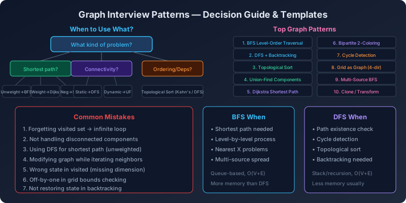
Graph problems appear in roughly 30-40% of technical interviews at top companies. The good news: most graph problems fit into a small number of recurring patterns. Master these patterns and you can solve the majority of graph questions you encounter.

The top 20 graph patterns

Pattern 1: Connected components

When: “How many groups/islands/clusters exist?”

Count distinct connected components using BFS, DFS, or Union-Find.

def count_components(n: int, edges: list[list[int]]) -> int:
    adj = [[] for _ in range(n)]
    for u, v in edges:
        adj[u].append(v)
        adj[v].append(u)

    visited = [False] * n
    count = 0

    def dfs(node):
        visited[node] = True
        for neighbor in adj[node]:
            if not visited[neighbor]:
                dfs(neighbor)

    for i in range(n):
        if not visited[i]:
            dfs(i)
            count += 1

    return count

Pattern 2: Shortest path (unweighted)

When: “Find the minimum number of steps/moves.”

Use BFS — it naturally finds shortest paths in unweighted graphs.

from collections import deque

def shortest_path(adj, src, dst):
    visited = {src}
    queue = deque([(src, 0)])

    while queue:
        node, dist = queue.popleft()
        if node == dst:
            return dist
        for neighbor in adj[node]:
            if neighbor not in visited:
                visited.add(neighbor)
                queue.append((neighbor, dist + 1))

    return -1  # unreachable

Pattern 3: Shortest path (weighted)

When: “Find minimum cost/distance with varying edge weights.”

Use Dijkstra’s for non-negative weights, Bellman-Ford if negative weights are possible.

import heapq

def dijkstra(adj, src, n):
    dist = [float('inf')] * n
    dist[src] = 0
    heap = [(0, src)]

    while heap:
        d, u = heapq.heappop(heap)
        if d > dist[u]:
            continue
        for v, w in adj[u]:
            if dist[u] + w < dist[v]:
                dist[v] = dist[u] + w
                heapq.heappush(heap, (dist[v], v))

    return dist

Pattern 4: Cycle detection

When: “Does a cycle exist?” or “Is it a valid tree?”

• Undirected graph: DFS with parent tracking or Union-Find.
• Directed graph: DFS with 3-color marking (white/gray/black).

def has_cycle_directed(adj, n):
    """3-color DFS cycle detection for directed graphs."""
    WHITE, GRAY, BLACK = 0, 1, 2
    color = [WHITE] * n

    def dfs(u):
        color[u] = GRAY
        for v in adj[u]:
            if color[v] == GRAY:
                return True     # back edge = cycle
            if color[v] == WHITE and dfs(v):
                return True
        color[u] = BLACK
        return False

    return any(color[i] == WHITE and dfs(i) for i in range(n))

Pattern 5: Topological sort

When: “Find a valid ordering of tasks with dependencies.”

Use Kahn’s algorithm (BFS) or DFS with post-order reversal.

from collections import deque

def topological_sort(adj, n):
    """Kahn's algorithm (BFS-based topological sort)."""
    in_degree = [0] * n
    for u in range(n):
        for v in adj[u]:
            in_degree[v] += 1

    queue = deque(v for v in range(n) if in_degree[v] == 0)
    order = []

    while queue:
        u = queue.popleft()
        order.append(u)
        for v in adj[u]:
            in_degree[v] -= 1
            if in_degree[v] == 0:
                queue.append(v)

    return order if len(order) == n else []  # empty = cycle exists

Pattern 6: Flood fill / grid traversal

When: Grid-based problems with connected regions.

Treat each cell as a node with 4 neighbors. Use DFS or BFS to explore the connected region.

Pattern 7: Bipartite check

When: “Can nodes be split into two groups with no same-group edges?”

BFS or DFS with 2-coloring.

def is_bipartite(adj, n):
    color = [-1] * n

    def bfs(start):
        color[start] = 0
        queue = deque([start])
        while queue:
            u = queue.popleft()
            for v in adj[u]:
                if color[v] == -1:
                    color[v] = 1 - color[u]
                    queue.append(v)
                elif color[v] == color[u]:
                    return False
        return True

    return all(color[i] != -1 or bfs(i) for i in range(n))

Pattern 8: Union-Find / dynamic connectivity

When: “Are these two elements connected?” with dynamic edge additions. Also used for grouping and merging sets.

Pattern 9: Minimum spanning tree

When: “Connect all nodes at minimum cost.” Use Kruskal (sparse) or Prim (dense).

Pattern 10: Shortest path with state

When: BFS/Dijkstra but the state includes more than just the node (e.g., keys collected, walls broken, fuel remaining).

def shortest_path_with_state(grid):
    """BFS with (row, col, state) as the node."""
    rows, cols = len(grid), len(grid[0])
    start = (0, 0, 0)       # (row, col, state_bitmask)
    visited = {start}
    queue = deque([(start, 0)])

    while queue:
        (r, c, state), dist = queue.popleft()
        # Check goal condition
        # Expand neighbors with updated state
        for dr, dc in [(0,1),(0,-1),(1,0),(-1,0)]:
            nr, nc = r + dr, c + dc
            if 0 <= nr < rows and 0 <= nc < cols:
                new_state = state  # update based on grid[nr][nc]
                if (nr, nc, new_state) not in visited:
                    visited.add((nr, nc, new_state))
                    queue.append(((nr, nc, new_state), dist + 1))

Pattern 11: Multi-source BFS

When: “Find distance from nearest X” for all cells simultaneously. Start BFS from all source cells at once.

Pattern 12: Backtracking on graphs

When: “Find all paths” or “find path with constraints.” DFS with explicit un-visiting.

Pattern 13: Eulerian path/circuit

When: “Use every edge exactly once.” Use Hierholzer’s algorithm.

Pattern 14: Strongly connected components

When: Directed graph decomposition. Use Tarjan’s or Kosaraju’s algorithm.

Pattern 15: Articulation points and bridges

When: “Which nodes/edges, if removed, disconnect the graph?” Use Tarjan’s bridge-finding algorithm.

Pattern 16: Network flow

When: Maximum flow, minimum cut, bipartite matching. Use Ford-Fulkerson or Dinic’s algorithm.

Pattern 17: Graph coloring

When: “Minimum colors so no adjacent nodes share a color.” Often reduces to bipartite check (2-coloring).

Pattern 18: Shortest path in DAG

When: Weighted DAG — topological sort + relaxation gives O(V + E), faster than Dijkstra.

Pattern 19: All-pairs shortest path

When: Need distances between all node pairs. Use Floyd-Warshall O(V^3).

Pattern 20: Implicit graphs

When: The graph is not given explicitly. States are nodes, valid transitions are edges. Examples: word ladder, sliding puzzle, open lock.

BFS vs DFS decision flowchart

Use this mental flowchart when you see a graph problem:

Step 1: What are you looking for?

• Shortest path -> BFS (unweighted) or Dijkstra (weighted)
• All reachable nodes -> Either works, DFS is simpler
• Cycle detection -> DFS (directed) or Union-Find (undirected)
• Topological order -> BFS (Kahn’s) or DFS (post-order)
• Connected components -> DFS, BFS, or Union-Find

Step 2: Are there constraints?

• Need level-by-level processing -> BFS
• Need to explore as deep as possible first -> DFS
• Dynamic edge additions -> Union-Find
• State beyond just the node -> BFS with state tuple

Step 3: Practical considerations

• Very deep graph, risk of stack overflow -> BFS or iterative DFS
• Need backtracking -> DFS
• Grid problems -> Either, but BFS is safer for large grids

When to use Union-Find

Union-Find excels in specific scenarios:

Use Union-Find when…	Do NOT use when…
Edges are added dynamically	You need shortest paths
You only care about connectivity, not paths	You need to traverse the graph
You need to merge groups efficiently	Edge weights matter for paths
Kruskal’s MST	Topological ordering needed
Checking if adding an edge creates a cycle	You need all paths

Union-Find template

class UnionFind:
    def __init__(self, n):
        self.parent = list(range(n))
        self.rank = [0] * n
        self.components = n

    def find(self, x):
        while self.parent[x] != x:
            self.parent[x] = self.parent[self.parent[x]]  # path compression
            x = self.parent[x]
        return x

    def union(self, x, y):
        rx, ry = self.find(x), self.find(y)
        if rx == ry:
            return False
        if self.rank[rx] < self.rank[ry]:
            rx, ry = ry, rx
        self.parent[ry] = rx
        if self.rank[rx] == self.rank[ry]:
            self.rank[rx] += 1
        self.components -= 1
        return True

    def connected(self, x, y):
        return self.find(x) == self.find(y)

Grid vs adjacency list

Criterion	Grid	Adjacency list
Input format	2D matrix	Edge list or adj list
Node identity	(row, col) pair	Integer or string
Neighbor access	4-directional offsets	adj[node]
Space	O(rows * cols)	O(V + E)
When to use	Matrix/board problems	General graph problems
Conversion	Not needed	Build from edge list

Grid to adjacency list conversion

Sometimes you need to convert a grid to an adjacency list (e.g., for Dijkstra on a weighted grid):

def grid_to_adj(grid):
    rows, cols = len(grid), len(grid[0])
    adj = [[] for _ in range(rows * cols)]

    for r in range(rows):
        for c in range(cols):
            node = r * cols + c
            for dr, dc in [(0, 1), (0, -1), (1, 0), (-1, 0)]:
                nr, nc = r + dr, c + dc
                if 0 <= nr < rows and 0 <= nc < cols:
                    neighbor = nr * cols + nc
                    adj[node].append((neighbor, grid[nr][nc]))

    return adj

BFS template

from collections import deque

def bfs_template(adj, start, n):
    """
    Standard BFS template.
    Returns: visited set, distance array, parent array.
    """
    visited = [False] * n
    dist = [-1] * n
    parent = [-1] * n

    visited[start] = True
    dist[start] = 0
    queue = deque([start])

    while queue:
        u = queue.popleft()
        for v in adj[u]:
            if not visited[v]:
                visited[v] = True
                dist[v] = dist[u] + 1
                parent[v] = u
                queue.append(v)

    return visited, dist, parent

DFS template (iterative)

def dfs_template(adj, start, n):
    """
    Iterative DFS template.
    Returns: visited set, discovery order.
    """
    visited = [False] * n
    order = []
    stack = [start]

    while stack:
        u = stack.pop()
        if visited[u]:
            continue
        visited[u] = True
        order.append(u)

        for v in adj[u]:
            if not visited[v]:
                stack.append(v)

    return visited, order

DFS template (recursive with timestamps)

def dfs_timestamps(adj, n):
    """
    DFS with entry/exit timestamps.
    Useful for subtree queries and LCA.
    """
    entry = [0] * n
    exit_time = [0] * n
    visited = [False] * n
    timer = [0]

    def dfs(u, parent=-1):
        visited[u] = True
        timer[0] += 1
        entry[u] = timer[0]

        for v in adj[u]:
            if not visited[v]:
                dfs(v, u)

        timer[0] += 1
        exit_time[u] = timer[0]

    for i in range(n):
        if not visited[i]:
            dfs(i)

    return entry, exit_time

Common mistakes in graph interviews

Mistake 1: marking visited after dequeue instead of before enqueue

Wrong:

# Marking after dequeue causes duplicate processing
while queue:
    node = queue.popleft()
    if node in visited:      # too late! node was added multiple times
        continue
    visited.add(node)
    for neighbor in adj[node]:
        queue.append(neighbor)  # may add same node many times

Right:

# Mark BEFORE adding to queue
while queue:
    node = queue.popleft()
    for neighbor in adj[node]:
        if neighbor not in visited:
            visited.add(neighbor)   # mark immediately
            queue.append(neighbor)

The wrong approach works but wastes time and space by processing the same node multiple times. In the worst case this can turn O(V + E) into O(V^2).

Mistake 2: using DFS for shortest path

DFS does NOT guarantee shortest path in an unweighted graph. Always use BFS for shortest path questions. DFS may find a path, but it will often not be the shortest one.

Mistake 3: not handling disconnected components

# Wrong: only processes one component
dfs(0)

# Right: process all components
for i in range(n):
    if not visited[i]:
        dfs(i)

This mistake is especially common in “count components” and “detect cycle” problems. If the graph is disconnected, a single DFS/BFS from node 0 misses entire components.

Mistake 4: wrong cycle detection in directed graphs

Using a simple visited set detects cross edges as cycles in directed graphs, producing false positives. Use 3-color marking:

• White (0): unvisited.
• Gray (1): currently in the DFS stack (being explored).
• Black (2): fully processed.

A cycle exists only when you encounter a gray node (back edge), not just any visited node.

Mistake 5: confusing node count with edge count

A tree with n nodes has n - 1 edges. A complete graph with n nodes has n * (n - 1) / 2 edges. Getting this wrong leads to off-by- one errors in loop bounds and tree validation.

Mistake 6: not considering edge cases

Always handle:

• Empty graph (n = 0)
• Single node (n = 1, no edges)
• No edges at all
• Self-loops
• Parallel edges (multigraph)
• Disconnected graph

Mistake 7: modifying the graph while iterating

When removing edges or nodes during traversal, iterate over a copy of the neighbor list, not the original. In Python:

# Wrong: modifying adj[u] while iterating
for v in adj[u]:
    adj[u].remove(v)

# Right: iterate over a copy
for v in list(adj[u]):
    adj[u].remove(v)

Interview strategy

1. Clarify the problem: Directed or undirected? Weighted or unweighted? Can there be cycles? Is the graph connected?

2. Identify the pattern: Match the problem to one of the 20 patterns above.

3. Choose the algorithm: Use the decision flowchart.

4. Build the graph: Convert the input to your preferred representation (adjacency list is almost always best).

5. Code the template: Start from your memorized BFS/DFS/UF template and adapt.

6. Handle edge cases: Empty input, single node, disconnected components.

7. State complexity: Clearly state time and space complexity after coding.

Big-O reference table

Algorithm	Time	Space	Use case
BFS	O(V + E)	O(V)	Shortest path (unweighted)
DFS	O(V + E)	O(V)	Traversal, cycle detection
Dijkstra	O(E log V)	O(V)	Shortest path (weighted)
Bellman-Ford	O(V * E)	O(V)	Negative weights
Floyd-Warshall	O(V^3)	O(V^2)	All-pairs shortest path
Topological Sort	O(V + E)	O(V)	DAG ordering
Union-Find	O(alpha(V))	O(V)	Dynamic connectivity
Kruskal	O(E log E)	O(V+E)	MST (sparse)
Prim	O(E log V)	O(V+E)	MST (dense)
Tarjan SCC	O(V + E)	O(V)	Strongly connected comp.

Practice problems by pattern

Connected components:

• Number of Islands - LeetCode 200
• Number of Provinces - LeetCode 547

Shortest path (unweighted):

• Word Ladder - LeetCode 127
• Open the Lock - LeetCode 752

Shortest path (weighted):

• Network Delay Time - LeetCode 743
• Path with Minimum Effort - LeetCode 1631

Topological sort:

• Course Schedule - LeetCode 207
• Course Schedule II - LeetCode 210

Cycle detection:

• Course Schedule - LeetCode 207
• Graph Valid Tree - LeetCode 261

Union-Find:

• Redundant Connection - LeetCode 684
• Accounts Merge - LeetCode 721

Grid traversal:

• Rotting Oranges - LeetCode 994
• Shortest Path in Binary Matrix - LeetCode 1091

State-based BFS:

• Shortest Path to Get All Keys - LeetCode 864
• Sliding Puzzle - LeetCode 773

Bipartite:

• Is Graph Bipartite - LeetCode 785
• Possible Bipartition - LeetCode 886

MST:

• Min Cost to Connect All Points - LeetCode 1584
• Connecting Cities With Minimum Cost - LeetCode 1135

Key takeaways

• Most graph interview problems fit one of 20 patterns. Identify the pattern first, then apply the matching algorithm.
• BFS for shortest paths, DFS for traversal and cycle detection, Union-Find for dynamic connectivity.
• Always mark nodes as visited before adding them to the queue in BFS to avoid duplicate processing.
• Use 3-color marking for cycle detection in directed graphs. A simple visited set produces false positives on cross edges.
• Memorize the BFS, DFS, and Union-Find templates. They are your starting point for nearly every graph problem.
• Clarify the problem constraints before coding: directed vs undirected, weighted vs unweighted, connected vs disconnected.
• Handle edge cases: empty graphs, single nodes, disconnected components, and self-loops.