Strongly Connected Components: Kosaraju and Tarjan

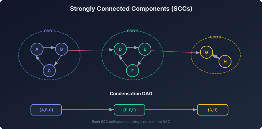
A strongly connected component (SCC) of a directed graph is a maximal set of nodes where every node can reach every other node in the set. In other words, for any two nodes u and v in the same SCC, there is a path from u to v and a path from v to u.

SCCs reveal the deep structure of directed graphs. Once you compute SCCs, you can collapse each one into a single super-node, creating a condensation DAG. This DAG exposes the high-level dependency structure that is hidden in the original graph.

Why SCCs Matter

Dependency analysis: In a dependency graph, an SCC represents a group of modules that depend on each other circularly. The condensation DAG shows the clean dependency ordering.

2-SAT: The implication graph of a 2-SAT problem is solved by finding SCCs. If a variable and its negation are in the same SCC, the formula is unsatisfiable.

Compiler optimization: SCCs in call graphs identify recursive function groups that must be compiled together.

Social networks: In a “follows” graph, an SCC represents a group where information can flow between all members.

Method 1: Kosaraju’s Algorithm

Kosaraju’s algorithm uses two DFS passes. The first pass on the original graph computes finish times. The second pass on the transposed (reversed) graph processes nodes in decreasing finish time order, and each DFS tree in the second pass is one SCC.

Why It Works

The key insight is about finish times and the transposed graph. If there is an edge from SCC X to SCC Y in the condensation DAG, then the last node to finish in X (during the first DFS) finishes after the last node in Y. In the transposed graph, the edge direction flips (Y to X), so starting from X in the second DFS cannot reach Y. This naturally separates the SCCs.

Implementation

def kosaraju(graph, num_nodes):
    """
    Find all SCCs using Kosaraju's algorithm.
    graph: dict or list of adjacency lists (directed)
    Returns: list of SCCs, each SCC is a list of nodes
    """
    # Step 1: DFS on original graph, record finish order
    visited = [False] * num_nodes
    finish_order = []

    def dfs1(node):
        visited[node] = True
        for neighbor in graph[node]:
            if not visited[neighbor]:
                dfs1(neighbor)
        finish_order.append(node)

    for i in range(num_nodes):
        if not visited[i]:
            dfs1(i)

    # Step 2: Build transposed graph
    transposed = [[] for _ in range(num_nodes)]
    for u in range(num_nodes):
        for v in graph[u]:
            transposed[v].append(u)

    # Step 3: DFS on transposed graph in reverse finish order
    visited = [False] * num_nodes
    sccs = []

    def dfs2(node, component):
        visited[node] = True
        component.append(node)
        for neighbor in transposed[node]:
            if not visited[neighbor]:
                dfs2(neighbor, component)

    for node in reversed(finish_order):
        if not visited[node]:
            component = []
            dfs2(node, component)
            sccs.append(component)

    return sccs

Example

# Directed graph with 3 SCCs
# SCC1: {0, 1, 2}, SCC2: {3, 4}, SCC3: {5}
graph = [
    [1],        # 0 -> 1
    [2],        # 1 -> 2
    [0, 3],     # 2 -> 0, 2 -> 3
    [4],        # 3 -> 4
    [3, 5],     # 4 -> 3, 4 -> 5
    []          # 5
]

sccs = kosaraju(graph, 6)
print(sccs)
# [[0, 2, 1], [3, 4], [5]]  (order may vary within each SCC)

Trace Through the Algorithm

First DFS (original graph):

• Start at 0: visit 0 -> 1 -> 2 -> 0 (visited), 3 -> 4 -> 3 (visited), 5. Finish order builds up: 5, 4, 3, 2, 1, 0.

Build transposed graph:

• Reverse all edges: 1->0, 2->1, 0->2, 3->2, 4->3, 3->4, 5->4.

Second DFS (transposed, reverse finish order):

• Process 0: DFS reaches 0->2->1. SCC = {0, 2, 1}.
• Process 3: DFS reaches 3->4. SCC = {3, 4}.
• Process 5: DFS reaches only 5. SCC = {5}.

Complexity

• Time: O(V + E) for both DFS passes
• Space: O(V + E) for the transposed graph

Method 2: Tarjan’s Algorithm

Tarjan’s algorithm finds SCCs in a single DFS pass. It uses two values for each node: the discovery time (disc) and the low-link value (low). The low-link value is the smallest discovery time reachable from the subtree rooted at that node.

A node is the root of an SCC if its low-link value equals its discovery time. When we find such a root, all nodes currently on the stack above it (including itself) form one SCC.

Implementation

def tarjan(graph, num_nodes):
    """
    Find all SCCs using Tarjan's algorithm.
    Single DFS pass with discovery times and low-link values.
    Returns: list of SCCs
    """
    disc = [-1] * num_nodes
    low = [-1] * num_nodes
    on_stack = [False] * num_nodes
    stack = []
    sccs = []
    timer = [0]  # Mutable counter

    def dfs(node):
        disc[node] = low[node] = timer[0]
        timer[0] += 1
        stack.append(node)
        on_stack[node] = True

        for neighbor in graph[node]:
            if disc[neighbor] == -1:
                # Unvisited: recurse
                dfs(neighbor)
                low[node] = min(low[node], low[neighbor])
            elif on_stack[neighbor]:
                # On stack: back edge, update low-link
                low[node] = min(low[node], disc[neighbor])

        # If node is root of SCC
        if low[node] == disc[node]:
            component = []
            while True:
                top = stack.pop()
                on_stack[top] = False
                component.append(top)
                if top == node:
                    break
            sccs.append(component)

    for i in range(num_nodes):
        if disc[i] == -1:
            dfs(i)

    return sccs

Example

graph = [
    [1],        # 0 -> 1
    [2],        # 1 -> 2
    [0, 3],     # 2 -> 0, 2 -> 3
    [4],        # 3 -> 4
    [3, 5],     # 4 -> 3, 4 -> 5
    []          # 5
]

sccs = tarjan(graph, 6)
print(sccs)
# [[5], [3, 4], [0, 1, 2]]  (bottom-up order)

Understanding Low-Link Values

The low-link value of a node is the key to Tarjan’s algorithm. It answers: what is the earliest discovered node that I can reach through my subtree, including back edges?

Node:  0  1  2  3  4  5
disc:  0  1  2  3  4  5
low:   0  0  0  3  3  5

Node 2 has low=0 because it can reach node 0 (disc=0) via the back edge 2->0. Node 1 inherits low=0 from node 2. Node 0 has disc=low=0, so it is the root of SCC 2. Node 4 has low=3 because it reaches node 3 (disc=3) via edge 4->3. Node 3 has disc=low=3, so it is the root of SCC 4. Node 5 has disc=low=5, so it is its own SCC.

Iterative Tarjan

For deep graphs that might overflow the recursion stack:

def tarjan_iterative(graph, num_nodes):
    """
    Iterative version of Tarjan's SCC algorithm.
    """
    disc = [-1] * num_nodes
    low = [-1] * num_nodes
    on_stack = [False] * num_nodes
    stack = []
    sccs = []
    timer = [0]

    for start in range(num_nodes):
        if disc[start] != -1:
            continue

        call_stack = [(start, 0)]  # (node, neighbor_index)
        disc[start] = low[start] = timer[0]
        timer[0] += 1
        stack.append(start)
        on_stack[start] = True

        while call_stack:
            node, idx = call_stack[-1]

            if idx < len(graph[node]):
                call_stack[-1] = (node, idx + 1)
                neighbor = graph[node][idx]

                if disc[neighbor] == -1:
                    disc[neighbor] = low[neighbor] = timer[0]
                    timer[0] += 1
                    stack.append(neighbor)
                    on_stack[neighbor] = True
                    call_stack.append((neighbor, 0))
                elif on_stack[neighbor]:
                    low[node] = min(low[node], disc[neighbor])
            else:
                # Done with this node
                if low[node] == disc[node]:
                    component = []
                    while True:
                        top = stack.pop()
                        on_stack[top] = False
                        component.append(top)
                        if top == node:
                            break
                    sccs.append(component)

                call_stack.pop()
                if call_stack:
                    parent = call_stack[-1][0]
                    low[parent] = min(low[parent], low[node])

    return sccs

Building the Condensation DAG

The condensation graph collapses each SCC into a single node and preserves edges between different SCCs. The result is always a DAG (no cycles, because if two super-nodes formed a cycle, their SCCs would merge into one larger SCC).

def build_condensation(graph, num_nodes, sccs):
    """
    Build the condensation DAG from SCCs.
    Returns: number of super-nodes, adjacency list of condensation,
             mapping from node to its SCC index
    """
    # Map each node to its SCC index
    node_to_scc = [0] * num_nodes
    for idx, scc in enumerate(sccs):
        for node in scc:
            node_to_scc[node] = idx

    # Build condensation adjacency list
    num_sccs = len(sccs)
    condensation = [set() for _ in range(num_sccs)]

    for u in range(num_nodes):
        for v in graph[u]:
            scc_u = node_to_scc[u]
            scc_v = node_to_scc[v]
            if scc_u != scc_v:
                condensation[scc_u].add(scc_v)

    # Convert sets to lists
    condensation = [list(s) for s in condensation]
    return num_sccs, condensation, node_to_scc

Example

graph = [
    [1], [2], [0, 3], [4], [3, 5], []
]
sccs = tarjan(graph, 6)
num_sccs, cond, mapping = build_condensation(graph, 6, sccs)

print(f"Number of SCCs: {num_sccs}")      # 3
print(f"Condensation: {cond}")             # [[1], [2], []]
print(f"Node to SCC: {mapping}")           # Maps each node to SCC index

Application: 2-SAT Solver

2-SAT is a satisfiability problem where each clause has exactly two literals. It can be solved in polynomial time using SCCs on the implication graph.

def solve_2sat(num_vars, clauses):
    """
    Solve 2-SAT using SCC.
    Variables: 0 to num_vars-1
    Negation of variable x is represented as x + num_vars
    clauses: list of (a, b) meaning (a OR b)
    Returns: assignment list or None if unsatisfiable
    """
    n = 2 * num_vars  # Variables and their negations

    def neg(x):
        return x + num_vars if x < num_vars else x - num_vars

    # Build implication graph
    # (a OR b) => (NOT a => b) AND (NOT b => a)
    graph = [[] for _ in range(n)]
    for a, b in clauses:
        graph[neg(a)].append(b)
        graph[neg(b)].append(a)

    sccs = tarjan(graph, n)

    # Check satisfiability: x and NOT x must be in different SCCs
    node_to_scc = [0] * n
    for idx, scc in enumerate(sccs):
        for node in scc:
            node_to_scc[node] = idx

    for x in range(num_vars):
        if node_to_scc[x] == node_to_scc[neg(x)]:
            return None  # Unsatisfiable

    # Assign values: variable is TRUE if its SCC comes after NOT x's SCC
    assignment = [False] * num_vars
    for x in range(num_vars):
        assignment[x] = node_to_scc[x] > node_to_scc[neg(x)]

    return assignment

Comparing Kosaraju and Tarjan

Feature	Kosaraju	Tarjan
DFS passes	2	1
Extra space	Transposed graph O(V+E)	Stack O(V)
Time	O(V+E)	O(V+E)
Implementation	Simpler to understand	More complex
Output order	Topological order of SCCs	Reverse topological
Online support	No (needs full graph twice)	Yes (single pass)

Kosaraju is easier to implement and understand. If you need to explain the algorithm in an interview, Kosaraju is usually the safer choice.

Tarjan is more efficient in practice because it only does one DFS pass and does not need to build the transposed graph. It is the preferred choice in competitive programming.

SCC-Based Reachability

Once you have the condensation DAG, many reachability questions become easier. For example, finding the minimum number of edges to add so that every node can reach every other node (making the whole graph one SCC).

def min_edges_to_strongly_connect(graph, num_nodes):
    """
    Find minimum edges to add to make the graph strongly connected.
    Answer: max(sources, sinks) in the condensation DAG.
    (Where sources have in-degree 0 and sinks have out-degree 0.)
    """
    sccs = tarjan(graph, num_nodes)

    if len(sccs) == 1:
        return 0  # Already strongly connected

    num_sccs, condensation, node_to_scc = build_condensation(
        graph, num_nodes, sccs
    )

    out_degree = [0] * num_sccs
    in_degree = [0] * num_sccs

    for u in range(num_sccs):
        for v in condensation[u]:
            out_degree[u] += 1
            in_degree[v] += 1

    sources = sum(1 for d in in_degree if d == 0)
    sinks = sum(1 for d in out_degree if d == 0)

    return max(sources, sinks)

Practice Problems

1. Kosaraju’s Algorithm (CSES) - Direct SCC computation
2. Critical Connections in a Network (LeetCode 1192) - Related bridge-finding
3. Satisfiability of Equality Equations (LeetCode 990) - Union-Find / SCC variant
4. 2-SAT problems (various competitive programming judges)
5. Reachability Queries after SCC condensation
6. Course Schedule IV (LeetCode 1462) - Reachability with condensation

Key Takeaways

Strongly connected components decompose a directed graph into its finest cyclical structure. Kosaraju uses two DFS passes (original graph, then transposed in reverse finish order) and is easy to understand. Tarjan uses one pass with discovery times and low-link values, which is more efficient. Both run in O(V + E) time.

The condensation DAG is the real prize. Once you collapse SCCs, you get a clean DAG where topological sort, reachability queries, and dependency analysis become straightforward. Many hard-looking graph problems become simple once you think in terms of SCCs and their condensation.