Advanced Graph Algorithms: SCCs, Flows & Bridges
Deep dive into advanced graph algorithms — Tarjan's and Kosaraju's for SCCs, bridges and articulation points, Euler paths, network flow, and 2-SAT with real-world applications.
What you'll learn
- ✓How to find strongly connected components with Tarjan's and Kosaraju's algorithms
- ✓How to identify bridges and articulation points in a graph
- ✓How to determine if a graph has an Euler path or circuit
- ✓How network flow works with Ford-Fulkerson and Edmonds-Karp
- ✓The min-cut / max-flow theorem and its applications
- ✓How to model and solve 2-SAT problems using SCCs
Prerequisites
- •Comfortable with Graphs Introduction and BFS/DFS
- •Familiar with Topological Sort
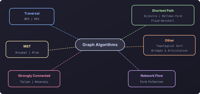
Basic graph algorithms — BFS, DFS, shortest paths, MST — solve a huge range of problems. But some questions need deeper machinery. Can you partition a network into its tightly-connected clusters? Can you find the single road whose removal disconnects a city? Can you push the maximum amount of water through a pipe network? This post covers the advanced graph algorithms that answer these questions.
1. Strongly Connected Components (SCCs)
In a directed graph, a strongly connected component is a maximal set of vertices where every vertex is reachable from every other vertex. Think of a group of friends where everyone follows everyone else on social media — that is an SCC.
(0) ──→ (1) ──→ (2)
↑ ↓ ↓
└──── (3) (4) ──→ (5)
↑ ↓
└───────┘
SCC 1: {0, 1, 3}
SCC 2: {2}
SCC 3: {4, 5}
Kosaraju’s Algorithm — two DFS passes
- First DFS: run DFS on the original graph, recording finish times (push to stack when done).
- Reverse all edges.
- Second DFS: pop vertices from the stack and DFS on the reversed graph. Each DFS tree is one SCC.
def kosaraju(n, adj):
    # adj[u] = list of neighbours of u
    visited = [False] * n
    order = []

    def dfs1(u):
        visited[u] = True
        for v in adj[u]:
            if not visited[v]:
                dfs1(v)
        order.append(u)

    # Step 1: fill order by finish time
    for i in range(n):
        if not visited[i]:
            dfs1(i)

    # Step 2: build reverse graph
    rev = [[] for _ in range(n)]
    for u in range(n):
        for v in adj[u]:
            rev[v].append(u)

    # Step 3: DFS on reverse in reverse finish order
    visited = [False] * n
    sccs = []

    def dfs2(u, comp):
        visited[u] = True
        comp.append(u)
        for v in rev[u]:
            if not visited[v]:
                dfs2(v, comp)

    for u in reversed(order):
        if not visited[u]:
            comp = []
            dfs2(u, comp)
            sccs.append(comp)

    return sccs
Time: O(V + E). Two linear DFS passes.
Tarjan’s Algorithm — single DFS pass
Tarjan’s algorithm finds SCCs in one DFS using a stack and two arrays: disc (discovery time) and low (lowest discovery time reachable).
def tarjan_scc(n, adj):
    disc = [-1] * n
    low = [0] * n
    on_stack = [False] * n
    stack = []
    timer = [0]
    sccs = []

    def dfs(u):
        disc[u] = low[u] = timer[0]
        timer[0] += 1
        stack.append(u)
        on_stack[u] = True

        for v in adj[u]:
            if disc[v] == -1:
                dfs(v)
                low[u] = min(low[u], low[v])
            elif on_stack[v]:
                low[u] = min(low[u], disc[v])

        # u is root of an SCC
        if low[u] == disc[u]:
            comp = []
            while True:
                v = stack.pop()
                on_stack[v] = False
                comp.append(v)
                if v == u:
                    break
            sccs.append(comp)

    for i in range(n):
        if disc[i] == -1:
            dfs(i)

    return sccs
When the low-link of a node equals its discovery time, it is the root of an SCC. Everything above it on the stack belongs to that SCC.
Real-world use: Kosaraju’s and Tarjan’s are used in compiler optimisation (finding dependency cycles), social network analysis (identifying tight communities), and solving 2-SAT (covered below).
2. Bridges and Articulation Points
A bridge is an edge whose removal disconnects the graph. An articulation point is a vertex whose removal disconnects the graph. Both are critical in network reliability analysis — “which cable, if cut, splits the network?”
Finding bridges with modified DFS
def find_bridges(n, adj):
    disc = [-1] * n
    low = [0] * n
    timer = [0]
    bridges = []

    def dfs(u, parent):
        disc[u] = low[u] = timer[0]
        timer[0] += 1

        for v in adj[u]:
            if v == parent:
                continue
            if disc[v] == -1:
                dfs(v, u)
                low[u] = min(low[u], low[v])
                if low[v] > disc[u]:
                    bridges.append((u, v))
            else:
                low[u] = min(low[u], disc[v])

    for i in range(n):
        if disc[i] == -1:
            dfs(i, -1)

    return bridges
The key condition: edge (u, v) is a bridge if low[v] > disc[u] — meaning v’s subtree has no back edge that reaches u or above.
Finding articulation points
def find_articulation_points(n, adj):
    disc = [-1] * n
    low = [0] * n
    timer = [0]
    ap = set()

    def dfs(u, parent):
        disc[u] = low[u] = timer[0]
        timer[0] += 1
        children = 0

        for v in adj[u]:
            if v == parent:
                continue
            if disc[v] == -1:
                children += 1
                dfs(v, u)
                low[u] = min(low[u], low[v])
                # Non-root with a child subtree that can't reach above u
                if parent != -1 and low[v] >= disc[u]:
                    ap.add(u)
            else:
                low[u] = min(low[u], disc[v])

        # Root with 2+ children
        if parent == -1 and children > 1:
            ap.add(u)

    for i in range(n):
        if disc[i] == -1:
            dfs(i, -1)

    return ap
Real-world: Internet backbone design — ISPs need to know which routers are articulation points so they can add redundant links.
3. Euler Paths and Circuits
An Euler circuit visits every edge exactly once and returns to the start. An Euler path visits every edge exactly once but may end at a different vertex. Think of the classic Konigsberg bridges problem.
When do they exist?
| Graph type | Euler circuit | Euler path |
|---|---|---|
| Undirected | Every vertex has even degree | Exactly 0 or 2 vertices have odd degree |
| Directed | Every vertex has in-degree = out-degree | At most one vertex has out - in = 1, at most one has in - out = 1 |
Hierholzer’s Algorithm
def euler_circuit(n, adj):
    # adj is adjacency list with mutable edge lists
    from collections import defaultdict, deque

    graph = defaultdict(deque)
    for u in range(n):
        for v in adj[u]:
            graph[u].append(v)

    stack = [0]
    circuit = []

    while stack:
        u = stack[-1]
        if graph[u]:
            v = graph[u].popleft()
            stack.append(v)
        else:
            circuit.append(stack.pop())

    circuit.reverse()
    return circuit
Time: O(E). The trick is that you greedily walk edges, and when you hit a dead end, you backtrack and insert detours.
Real-world: Route planning for mail delivery, street sweeping, and DNA fragment assembly in bioinformatics (Euler paths on de Bruijn graphs).
4. Network Flow — Ford-Fulkerson and Edmonds-Karp
Imagine a network of water pipes. Each pipe has a capacity. You want to push the maximum volume of water from a source to a sink. This is the maximum flow problem.
10        10
(S) ──────→ (A) ──────→ (T)
│            │  ↗         ↑
│ 10      5  │ / 15       │ 10
↓            ↓/           │
(B) ──────→ (C) ──────────┘
15
Ford-Fulkerson Method
- While there exists an augmenting path from source to sink in the residual graph:
- Find the bottleneck (minimum residual capacity along the path)
- Push that much flow along the path
- Update residual capacities
The residual graph has forward edges (remaining capacity) and backward edges (flow that can be “undone”).
Edmonds-Karp: BFS-based Ford-Fulkerson
Using BFS to find augmenting paths guarantees O(V * E^2) time — polynomial, unlike plain Ford-Fulkerson which can be slow with irrational capacities.
from collections import deque

def edmonds_karp(n, capacity, source, sink):
    """
    capacity[u][v] = capacity of edge u -> v
    Returns maximum flow value.
    """
    flow = [[0] * n for _ in range(n)]
    total_flow = 0

    while True:
        # BFS to find augmenting path
        parent = [-1] * n
        parent[source] = source
        queue = deque([source])

        while queue and parent[sink] == -1:
            u = queue.popleft()
            for v in range(n):
                if parent[v] == -1 and capacity[u][v] - flow[u][v] > 0:
                    parent[v] = u
                    queue.append(v)

        if parent[sink] == -1:
            break  # no augmenting path

        # Find bottleneck
        bottleneck = float('inf')
        v = sink
        while v != source:
            u = parent[v]
            bottleneck = min(bottleneck, capacity[u][v] - flow[u][v])
            v = u

        # Update flow
        v = sink
        while v != source:
            u = parent[v]
            flow[u][v] += bottleneck
            flow[v][u] -= bottleneck
            v = u

        total_flow += bottleneck

    return total_flow

# Example
n = 4  # S=0, A=1, B=2, T=3
cap = [[0]*4 for _ in range(4)]
cap[0][1] = 10
cap[0][2] = 10
cap[1][2] = 5
cap[1][3] = 10
cap[2][3] = 15
print(edmonds_karp(4, cap, 0, 3))  # 20
5. Min-Cut / Max-Flow Theorem
One of the most elegant results in graph theory:
The maximum flow from source to sink equals the minimum capacity of a cut that separates source from sink.
A cut is a partition of vertices into two sets S (containing source) and T (containing sink). The capacity of the cut is the sum of capacities of edges going from S to T.
After running max-flow, the min-cut can be found by doing BFS/DFS from the source in the residual graph. Vertices reachable from source are in S; the rest are in T.
Applications:
- Image segmentation: pixels are nodes, edges encode similarity. Min-cut separates foreground from background.
- Airline scheduling: matching flights to crews.
- Bipartite matching: maximum matching in a bipartite graph reduces to max-flow.
6. The 2-SAT Problem
Given a boolean formula in 2-CNF (each clause has exactly 2 literals), determine if it is satisfiable.
Example: (x1 OR x2) AND (NOT x1 OR x3) AND (NOT x2 OR NOT x3)
The implication graph approach
Each clause (a OR b) becomes two implications: NOT a → b and NOT b → a. Build a directed graph of these implications, then find SCCs using Tarjan’s.
Key insight: the formula is unsatisfiable if and only if some variable x and its negation NOT x are in the same SCC (a contradiction: x implies NOT x and NOT x implies x).
def solve_2sat(n, clauses):
    """
    n = number of variables (0-indexed)
    clauses = list of (a, b) where each is a literal:
      variable i is represented as 2*i (true) and 2*i+1 (false)
    """
    adj = [[] for _ in range(2 * n)]

    def neg(x):
        return x ^ 1

    for a, b in clauses:
        # (a OR b) => (NOT a -> b) AND (NOT b -> a)
        adj[neg(a)].append(b)
        adj[neg(b)].append(a)

    # Find SCCs using Tarjan's
    sccs = tarjan_scc(2 * n, adj)

    # Assign component IDs
    comp = [0] * (2 * n)
    for idx, scc in enumerate(sccs):
        for node in scc:
            comp[node] = idx

    # Check satisfiability
    for i in range(n):
        if comp[2 * i] == comp[2 * i + 1]:
            return None  # unsatisfiable

    # Determine assignment: variable is TRUE if comp[x] > comp[NOT x]
    # (Tarjan's returns SCCs in reverse topological order)
    assignment = [comp[2 * i] > comp[2 * i + 1] for i in range(n)]
    return assignment
Real-world: 2-SAT appears in circuit design, scheduling with constraints (“if task A is morning, then task B must be afternoon”), and configuration management.
Algorithm Selection Guide
| Problem | Algorithm | Time |
|---|---|---|
| Find tightly-connected clusters in directed graph | Tarjan’s / Kosaraju’s SCC | O(V + E) |
| Find critical edges/nodes | Bridges / Articulation Points | O(V + E) |
| Visit every edge exactly once | Euler Path (Hierholzer’s) | O(E) |
| Maximum flow through a network | Edmonds-Karp | O(V * E^2) |
| Minimum cut of a network | Max-flow + BFS | O(V * E^2) |
| Boolean satisfiability with 2 literals per clause | 2-SAT via SCC | O(V + E) |
Recap
These advanced graph algorithms unlock a new tier of problem-solving:
- SCCs decompose directed graphs into their fundamental building blocks
- Bridges and articulation points reveal vulnerabilities in networks
- Euler paths solve traversal problems where every edge matters
- Network flow models capacity-constrained routing, matching, and assignment
- 2-SAT solves constraint satisfaction by reducing it to graph reachability
Each algorithm builds on the DFS framework you already know. The conceptual leap is not in the code — it is in recognising which graph model fits the problem.
Next steps
See how these graph structures appear in real systems in DSA in Real Systems, or explore more competitive programming patterns in CP Patterns.
Questions or feedback? Email codeloomdevv@gmail.com.
Related articles
- DSA Alien Dictionary: Topological Sort from Word Ordering
Derive character ordering from sorted alien words using topological sort, with course schedule variants and prerequisite chain problems.
- DSA Detecting Negative Cycles in Graphs
Learn how to detect negative cycles using Bellman-Ford's nth relaxation, SPFA algorithm, and apply it to arbitrage detection in currency exchange graphs.
- DSA Word Search, Boggle Solver, and Word Ladder: Grid + String Graph Problems
Solve word search with DFS backtracking, Boggle with Trie pruning, and word ladder with BFS for efficient string transformation problems.
- DSA A* Search Algorithm: Heuristic Pathfinding Explained
Learn the A* search algorithm with f=g+h, admissible heuristics, grid pathfinding, and Python implementation compared to Dijkstra and BFS.