Data Warehouse Concepts: Star Schema and Beyond

A data warehouse is a database designed for analytical queries, not for running your application. Your app’s PostgreSQL database is optimized for fast single-row lookups and transactional writes. A warehouse is optimized for scanning millions of rows, aggregating columns, and answering questions like “what was our revenue by region last quarter?”

OLTP vs OLAP

Two acronyms that define the split:

Property	OLTP (Transactional)	OLAP (Analytical)
Purpose	Run the application	Answer business questions
Queries	Simple, touch few rows	Complex, scan millions of rows
Schema	Normalized (3NF)	Denormalized (star/snowflake)
Writes	Many small inserts/updates	Bulk loads, append-mostly
Users	Application servers	Analysts, dashboards, ML pipelines
Examples	PostgreSQL, MySQL	Snowflake, BigQuery, Redshift

You never run analytical queries against your production OLTP database. It would slow down the application and the queries themselves would be painful to write against a normalized schema with dozens of joins. That is why warehouses exist.

Star schema

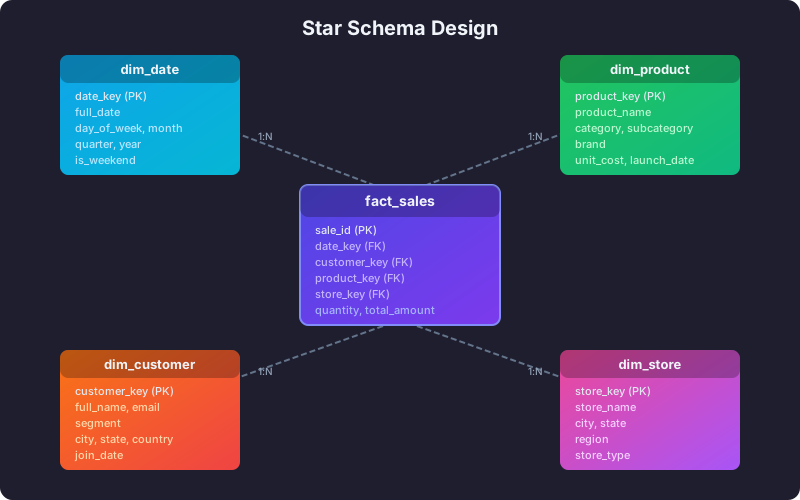
The star schema is the most common warehouse design pattern. It places a fact table at the center, surrounded by dimension tables — one join away.

Fact tables

A fact table records measurable business events. Each row represents something that happened — a sale, a click, a shipment, a payment.

CREATE TABLE fact_sales (
    sale_id         BIGINT PRIMARY KEY,
    date_key        INT REFERENCES dim_date(date_key),
    customer_key    INT REFERENCES dim_customer(customer_key),
    product_key     INT REFERENCES dim_product(product_key),
    store_key       INT REFERENCES dim_store(store_key),
    quantity        INT,
    unit_price      DECIMAL(10, 2),
    discount_amount DECIMAL(10, 2),
    total_amount    DECIMAL(12, 2)
);

The numeric columns (quantity, unit_price, total_amount) are measures — the things you aggregate. The key columns link to dimensions that provide context.

Types of fact tables:

• Transaction fact — one row per event. Most common. Each sale, each click.
• Periodic snapshot — one row per time period. Daily account balance, monthly inventory level.
• Accumulating snapshot — one row per lifecycle. An order row that updates as it moves through created → shipped → delivered.

Measure additivity:

• Additive — can sum across all dimensions. Revenue, quantity.
• Semi-additive — can sum across some dimensions but not time. Account balance (summing across months makes no sense).
• Non-additive — cannot be summed. Ratios, percentages, averages. Store the components and compute at query time.

Dimension tables

Dimension tables describe the who, what, where, when of a business event. They are typically wide (many columns) and short (thousands to millions of rows, not billions).

CREATE TABLE dim_product (
    product_key   INT PRIMARY KEY,
    product_id    VARCHAR(20),
    product_name  VARCHAR(200),
    category      VARCHAR(100),
    subcategory   VARCHAR(100),
    brand         VARCHAR(100),
    unit_cost     DECIMAL(10, 2),
    launch_date   DATE
);

CREATE TABLE dim_date (
    date_key      INT PRIMARY KEY,
    full_date     DATE,
    day_of_week   VARCHAR(10),
    month_name    VARCHAR(10),
    quarter       INT,
    year          INT,
    is_weekend    BOOLEAN,
    fiscal_quarter INT
);

CREATE TABLE dim_customer (
    customer_key  INT PRIMARY KEY,
    customer_id   VARCHAR(20),
    full_name     VARCHAR(200),
    email         VARCHAR(200),
    segment       VARCHAR(50),
    city          VARCHAR(100),
    state         VARCHAR(100),
    country       VARCHAR(100),
    join_date     DATE
);

Notice product_key vs product_id. The surrogate key (product_key) is a warehouse-generated integer. The natural key (product_id) is the business identifier from the source system. Always use surrogate keys as primary keys in the warehouse — they handle slowly changing dimensions and protect against source system key collisions.

Querying a star schema

The beauty of a star schema is simple, readable queries:

SELECT
    d.year,
    d.quarter,
    p.category,
    c.segment,
    SUM(f.total_amount)    AS revenue,
    SUM(f.quantity)         AS units_sold,
    COUNT(DISTINCT f.customer_key) AS unique_customers
FROM fact_sales f
JOIN dim_date d     ON f.date_key = d.date_key
JOIN dim_product p  ON f.product_key = p.product_key
JOIN dim_customer c ON f.customer_key = c.customer_key
WHERE d.year = 2026
GROUP BY d.year, d.quarter, p.category, c.segment
ORDER BY revenue DESC;

One fact table, a few joins, and you have revenue by quarter, category, and customer segment. BI tools like Looker, Tableau, and Metabase are designed to generate exactly this kind of query.

Snowflake schema

A snowflake schema normalizes the dimension tables. Instead of one dim_product table with a category column, you split it into dim_product → dim_category → dim_department.

CREATE TABLE dim_category (
    category_key   INT PRIMARY KEY,
    category_name  VARCHAR(100),
    department_key INT REFERENCES dim_department(department_key)
);

CREATE TABLE dim_product (
    product_key   INT PRIMARY KEY,
    product_name  VARCHAR(200),
    category_key  INT REFERENCES dim_category(category_key),
    brand_key     INT REFERENCES dim_brand(brand_key),
    unit_cost     DECIMAL(10, 2)
);

Trade-offs:

• Snowflake schemas use less storage (no repeated category names in every product row).
• Star schemas are faster and simpler to query (fewer joins).
• Modern columnar warehouses compress repeated values extremely well, so the storage advantage of snowflake schemas is minimal.

In practice, most teams use star schemas. The query simplicity and BI tool compatibility outweigh the marginal storage savings.

Slowly changing dimensions (SCD)

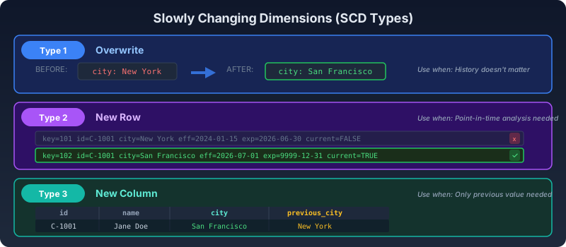
Dimensions change over time. A customer moves cities. A product changes categories. How you handle these changes defines your SCD type.

SCD Type 1 — Overwrite

Simply overwrite the old value. No history preserved.

UPDATE dim_customer
SET city = 'San Francisco', state = 'California'
WHERE customer_id = 'C-1001';

Use when: history does not matter. The customer’s current city is all you need.

SCD Type 2 — Add a new row

Create a new row with the updated values. Mark the old row as expired.

-- Old row (now expired)
-- customer_key=101, customer_id='C-1001', city='New York',
--   effective_date='2024-01-15', expiry_date='2026-06-30', is_current=FALSE

-- New row
INSERT INTO dim_customer (customer_key, customer_id, full_name, city, state,
                          effective_date, expiry_date, is_current)
VALUES (102, 'C-1001', 'Jane Doe', 'San Francisco', 'California',
        '2026-07-01', '9999-12-31', TRUE);

Use when: you need to analyze data as it was at a point in time. “What was our revenue by customer city in Q1?” should use the city the customer lived in during Q1, not their current city.

SCD Type 3 — Add a column

Add a previous_city column alongside the current one.

ALTER TABLE dim_customer ADD COLUMN previous_city VARCHAR(100);

UPDATE dim_customer
SET previous_city = city, city = 'San Francisco'
WHERE customer_id = 'C-1001';

Use when: you only need the previous value, not full history. Rarely used in practice — Type 2 is more flexible.

Performance techniques

Partitioning

Split a large table into segments based on a column — typically date.

-- BigQuery example
CREATE TABLE fact_events
PARTITION BY DATE(event_timestamp)
AS SELECT * FROM raw_events;

Queries that filter on event_timestamp only scan the relevant partitions. A query for January data skips all other months entirely.

Clustering

Within each partition, sort the data by frequently filtered columns.

-- BigQuery example
CREATE TABLE fact_events
PARTITION BY DATE(event_timestamp)
CLUSTER BY customer_id, event_type
AS SELECT * FROM raw_events;

A query filtering on customer_id = 'C-1001' now scans a tiny fraction of each partition.

Materialized views

Pre-compute expensive aggregations and refresh them on schedule.

-- Snowflake example
CREATE MATERIALIZED VIEW mv_daily_revenue AS
SELECT
    date_key,
    SUM(total_amount) AS daily_revenue,
    COUNT(*) AS num_transactions
FROM fact_sales
GROUP BY date_key;

Dashboards querying daily revenue now read from the materialized view instead of scanning the full fact table.

Next steps

• ETL vs ELT Pipelines — how data gets into the warehouse.
• Data Lakes vs Warehouses vs Lakehouses — the broader storage landscape.
• What Is Apache Airflow? — schedule your warehouse loads.