Data Partitioning Strategies for Scale

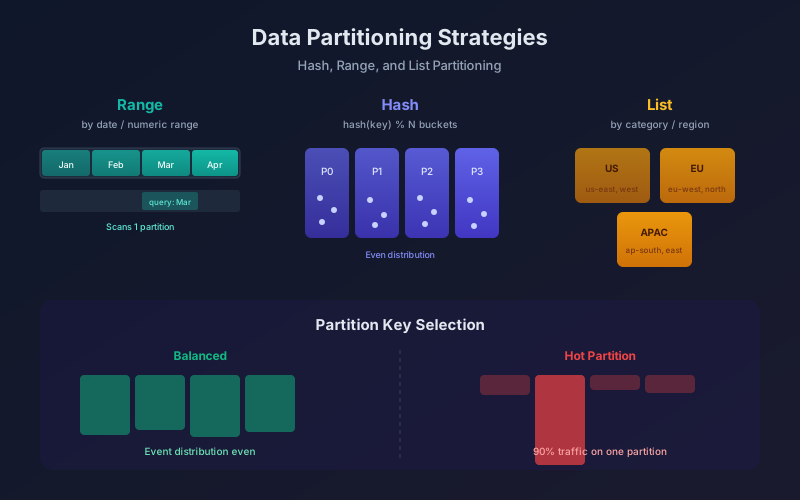
Partitioning splits a large dataset into smaller, independent chunks that can be stored, queried, and managed separately. It is the single most impactful decision for query performance at scale. Get it right and queries scan megabytes instead of terabytes. Get it wrong and you have hot partitions, skewed joins, and angry on-call engineers.

Why partition?

Without partitioning, a query against a 10TB table scans all 10TB. With date partitioning, a query for yesterday’s data scans only that day’s partition — maybe 30GB. That is a 300x reduction in data scanned, which translates directly to faster queries and lower compute costs.

-- Without partitioning: scans entire table (10 TB)
SELECT COUNT(*) FROM events WHERE event_date = '2026-08-08';

-- With date partitioning: scans one partition (~30 GB)
SELECT COUNT(*) FROM events WHERE event_date = '2026-08-08';
-- Same SQL, but the engine knows to skip 99.7% of the data

The three partitioning strategies

1. Range partitioning

Data is split based on a continuous range of values — typically dates or numeric IDs.

-- PostgreSQL range partitioning
CREATE TABLE events (
    id          BIGINT,
    event_date  DATE NOT NULL,
    user_id     BIGINT,
    event_type  TEXT,
    payload     JSONB
) PARTITION BY RANGE (event_date);

CREATE TABLE events_2026_07 PARTITION OF events
    FOR VALUES FROM ('2026-07-01') TO ('2026-08-01');

CREATE TABLE events_2026_08 PARTITION OF events
    FOR VALUES FROM ('2026-08-01') TO ('2026-09-01');

In BigQuery and Spark, range partitioning on date is the default pattern:

-- BigQuery
CREATE TABLE project.dataset.events (
    id INT64,
    event_date DATE,
    user_id INT64,
    event_type STRING
)
PARTITION BY event_date
CLUSTER BY user_id;

Best for: Time-series data, logs, events — any workload where queries filter by date range.

Watch out for: If recent partitions get far more writes than old ones, you get write skew. A “today” partition handling 90% of inserts while 364 other partitions sit idle.

2. Hash partitioning

A hash function distributes rows evenly across a fixed number of partitions. The engine computes hash(partition_key) % num_partitions to decide where each row goes.

-- PostgreSQL hash partitioning
CREATE TABLE user_profiles (
    user_id     BIGINT NOT NULL,
    username    TEXT,
    email       TEXT,
    created_at  TIMESTAMP
) PARTITION BY HASH (user_id);

CREATE TABLE user_profiles_p0 PARTITION OF user_profiles
    FOR VALUES WITH (MODULUS 4, REMAINDER 0);
CREATE TABLE user_profiles_p1 PARTITION OF user_profiles
    FOR VALUES WITH (MODULUS 4, REMAINDER 1);
CREATE TABLE user_profiles_p2 PARTITION OF user_profiles
    FOR VALUES WITH (MODULUS 4, REMAINDER 2);
CREATE TABLE user_profiles_p3 PARTITION OF user_profiles
    FOR VALUES WITH (MODULUS 4, REMAINDER 3);

Best for: Even distribution of reads and writes. Point lookups by key (WHERE user_id = 12345).

Watch out for: Range queries become expensive — WHERE user_id BETWEEN 1000 AND 2000 must scan all partitions because hash destroys ordering.

3. List partitioning

Data is split based on a predefined list of discrete values.

-- PostgreSQL list partitioning
CREATE TABLE orders (
    id          BIGINT,
    region      TEXT NOT NULL,
    amount      NUMERIC,
    order_date  DATE
) PARTITION BY LIST (region);

CREATE TABLE orders_us PARTITION OF orders
    FOR VALUES IN ('us-east', 'us-west', 'us-central');
CREATE TABLE orders_eu PARTITION OF orders
    FOR VALUES IN ('eu-west', 'eu-central', 'eu-north');
CREATE TABLE orders_apac PARTITION OF orders
    FOR VALUES IN ('ap-south', 'ap-east', 'ap-southeast');

Best for: Multi-tenant systems, geographic data, categorical dimensions.

Watch out for: Uneven category sizes cause skew. If 80% of orders come from us-east, the US partition does most of the work.

Choosing a partition key

The partition key is the column (or columns) the engine uses to assign rows to partitions. This choice determines query performance, write distribution, and join efficiency.

Rules of thumb

1. Pick columns that appear in WHERE clauses. If 90% of queries filter by event_date, partition by event_date.

2. Pick columns with moderate cardinality. Too few distinct values (e.g., status with 3 values) creates too few partitions. Too many (e.g., user_id with 100M values) creates too many small files.

3. Match the partition key to your join keys. If you frequently join orders and order_items on order_date, partitioning both by order_date enables partition-wise joins — the engine joins matching partitions independently.

4. Consider write distribution. If all writes go to the same partition, you create a bottleneck.

Compound partition keys

Sometimes one column is not enough. Use composite partitioning:

-- Hive / Spark: partition by date and region
CREATE TABLE events (
    event_id    BIGINT,
    event_type  STRING,
    payload     STRING
)
PARTITIONED BY (event_date STRING, region STRING)
STORED AS PARQUET;

-- This creates a directory structure:
-- events/event_date=2026-08-09/region=us-east/
-- events/event_date=2026-08-09/region=eu-west/

The hot partition problem

A hot partition is one that receives disproportionately more traffic than others. It is the most common partitioning mistake.

Example: partitioning by customer_id in a B2B SaaS

If one enterprise customer generates 60% of your events, the partition holding that customer becomes a bottleneck while other partitions sit idle.

Solutions

Add a salt (random suffix):

import hashlib

def salted_key(customer_id: str, num_buckets: int = 8) -> str:
    """Add a salt to spread a hot key across multiple partitions."""
    salt = int(hashlib.md5(customer_id.encode()).hexdigest(), 16) % num_buckets
    return f"{customer_id}_{salt}"

# customer_123 → customer_123_0, customer_123_1, ..., customer_123_7
# Writes spread across 8 partitions instead of 1
# Reads must query all 8 and merge

Use a composite key: Partition by (customer_id, event_hour) so a single customer’s data spreads across hourly sub-partitions.

Repartition periodically: In Spark, call repartition() before writing to rebalance skewed data:

df = spark.read.parquet("s3://lake/raw/events/")

# Before writing, repartition to avoid skew
df.repartition(200, "event_date") \
  .write.partitionBy("event_date") \
  .parquet("s3://lake/processed/events/")

Partitioning in data warehouses

Modern warehouses handle partitioning differently from traditional databases.

BigQuery

Supports date/timestamp partitioning and integer range partitioning. Combine with clustering for further pruning:

CREATE TABLE analytics.page_views (
    view_id     INT64,
    user_id     INT64,
    page_url    STRING,
    view_time   TIMESTAMP,
    country     STRING
)
PARTITION BY DATE(view_time)
CLUSTER BY country, user_id;

Queries filtering by view_time prune partitions. Within each partition, clustering sorts by country then user_id, enabling block-level pruning.

Snowflake

Snowflake uses micro-partitions automatically — small (50-500MB) compressed column files. You influence partition pruning through clustering keys:

ALTER TABLE events CLUSTER BY (event_date, region);

Snowflake recluters data in the background. You do not manually create partitions.

Apache Iceberg

Iceberg supports hidden partitioning — transforms on columns without changing the schema:

CREATE TABLE catalog.events (
    id          BIGINT,
    event_time  TIMESTAMP,
    user_id     BIGINT,
    event_type  STRING
)
USING iceberg
PARTITIONED BY (days(event_time), bucket(16, user_id));

Queries filter on event_time directly. Iceberg translates the filter to partition pruning automatically — users never see the partition column.

Anti-patterns to avoid

1. Over-partitioning. Creating millions of tiny partitions (one per user_id) causes metadata overhead and small-file problems. Aim for partitions between 128MB and 1GB.

2. Partitioning by a column nobody queries. If you partition by created_at but every query filters by customer_id, you scan all partitions every time.

3. Ignoring partition pruning in joins. If your fact table is partitioned by date but your join does not include date, the engine scans the entire fact table.

4. Forgetting to add new partitions. In range-partitioned PostgreSQL tables, rows that do not match any partition are rejected. Automate partition creation.

Key takeaways

• Range partitioning for time-series workloads. It is the most common and most effective strategy.
• Hash partitioning for even distribution and point lookups.
• List partitioning for categorical splits like region or tenant.
• Pick partition keys that match your query patterns — this is more important than the partitioning type.
• Monitor for hot partitions and use salting or composite keys to mitigate skew.

Next steps

• Data Warehouse Concepts — where partitioning meets warehouse architecture.
• Dimensional Modeling Deep Dive — how to model the data that sits inside these partitions.
• Apache Iceberg: The Modern Table Format — hidden partitioning and schema evolution.