Shortest Path Algorithms: BFS, Dijkstra, Bellman-Ford, Floyd-Warshall

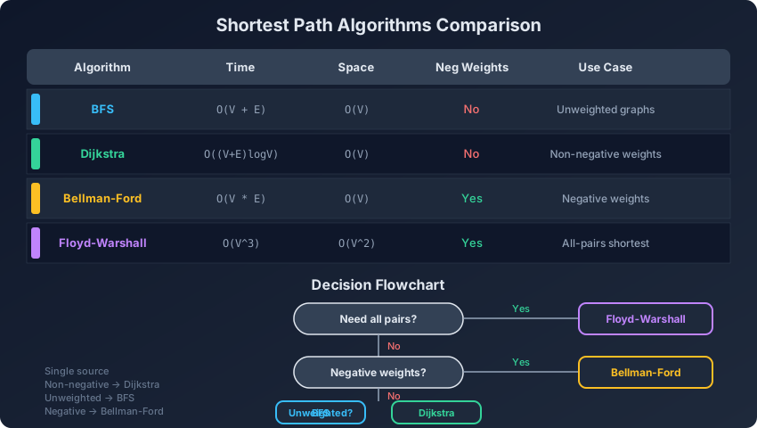
Shortest path problems appear everywhere in software engineering: routing packets across networks, GPS navigation, social network degrees of separation, and game pathfinding. The right algorithm depends on three questions: Are the edge weights all equal? Can weights be negative? Do you need paths between all pairs of nodes?

This article covers all four classical shortest path algorithms side by side. Each section includes the core idea, a clean Python implementation, complexity analysis, and guidance on when to use it.

The Decision Framework

Before diving into code, here is how to pick the right algorithm:

1. Unweighted graph? Use BFS. It is the simplest and fastest.
2. Weighted, no negative edges, single source? Use Dijkstra. It is the standard.
3. Negative edge weights possible? Use Bellman-Ford. It also detects negative cycles.
4. Need shortest path between every pair of nodes? Use Floyd-Warshall.

Algorithm 1: BFS for Unweighted Graphs

When all edges have the same weight (or weight 1), BFS naturally finds the shortest path. The first time BFS reaches a node, that is the shortest distance because BFS explores nodes level by level.

from collections import deque

def bfs_shortest_path(graph, source):
    """
    Find shortest paths from source to all nodes in an unweighted graph.
    graph: dict mapping node -> list of neighbors
    Returns: dict of distances, dict of parents for path reconstruction
    """
    dist = {source: 0}
    parent = {source: None}
    queue = deque([source])

    while queue:
        node = queue.popleft()
        for neighbor in graph[node]:
            if neighbor not in dist:
                dist[neighbor] = dist[node] + 1
                parent[neighbor] = node
                queue.append(neighbor)

    return dist, parent


def reconstruct_path(parent, target):
    """Reconstruct shortest path from source to target."""
    path = []
    current = target
    while current is not None:
        path.append(current)
        current = parent[current]
    return path[::-1]

Example

graph = {
    'A': ['B', 'C'],
    'B': ['A', 'D', 'E'],
    'C': ['A', 'F'],
    'D': ['B'],
    'E': ['B', 'F'],
    'F': ['C', 'E']
}

dist, parent = bfs_shortest_path(graph, 'A')
print(dist)    # {'A': 0, 'B': 1, 'C': 1, 'D': 2, 'E': 2, 'F': 2}

path = reconstruct_path(parent, 'F')
print(path)    # ['A', 'C', 'F']

Complexity

• Time: O(V + E)
• Space: O(V)
• Best for: Unweighted graphs, grid problems, social network distance

Algorithm 2: Dijkstra’s Algorithm

Dijkstra handles weighted graphs with non-negative edge weights. It greedily selects the unvisited node with the smallest tentative distance, finalizes it, and relaxes all its outgoing edges.

The greedy choice works because edge weights are non-negative. Once you pop a node from the priority queue with some distance d, no other path to that node can be shorter, since any detour adds non-negative weight.

import heapq
from math import inf

def dijkstra(graph, source):
    """
    Find shortest paths from source to all nodes.
    graph: dict mapping node -> list of (neighbor, weight) tuples
    Returns: dict of distances, dict of parents
    """
    dist = {node: inf for node in graph}
    dist[source] = 0
    parent = {node: None for node in graph}
    visited = set()
    pq = [(0, source)]

    while pq:
        d, node = heapq.heappop(pq)

        if node in visited:
            continue
        visited.add(node)

        for neighbor, weight in graph[node]:
            new_dist = d + weight
            if new_dist < dist[neighbor]:
                dist[neighbor] = new_dist
                parent[neighbor] = node
                heapq.heappush(pq, (new_dist, neighbor))

    return dist, parent

Example

graph = {
    'A': [('B', 4), ('C', 2)],
    'B': [('A', 4), ('D', 3), ('E', 1)],
    'C': [('A', 2), ('B', 1), ('F', 5)],
    'D': [('B', 3)],
    'E': [('B', 1), ('F', 2)],
    'F': [('C', 5), ('E', 2)]
}

dist, parent = dijkstra(graph, 'A')
print(dist)
# {'A': 0, 'B': 3, 'C': 2, 'D': 6, 'E': 4, 'F': 6}

path = reconstruct_path(parent, 'F')
print(path)  # ['A', 'C', 'B', 'E', 'F']

Why Negative Weights Break Dijkstra

Consider three nodes: A to B with weight 1, A to C with weight 5, C to B with weight -10. Dijkstra visits B first with distance 1 and finalizes it. But the path A to C to B has distance 5 + (-10) = -5, which is shorter. Since B is already finalized, Dijkstra misses this.

# This gives WRONG results with Dijkstra!
broken_graph = {
    'A': [('B', 1), ('C', 5)],
    'B': [],
    'C': [('B', -10)]
}
# Dijkstra says dist[B] = 1, but actual shortest is -5

Complexity

• Time: O((V + E) log V) with a binary heap
• Space: O(V)
• Best for: Weighted graphs with non-negative weights, road networks, GPS

Dijkstra Variants

Lazy Dijkstra (shown above) pushes duplicate entries into the heap and skips stale ones. This is the simplest implementation.

Eager Dijkstra uses a decrease-key operation to update priorities in place, avoiding duplicates. Python’s heapq does not support decrease-key natively, so lazy Dijkstra is standard in Python.

def dijkstra_with_early_exit(graph, source, target):
    """
    Dijkstra with early termination when target is reached.
    Useful when you only need the distance to one specific node.
    """
    dist = {node: inf for node in graph}
    dist[source] = 0
    visited = set()
    pq = [(0, source)]

    while pq:
        d, node = heapq.heappop(pq)

        if node == target:
            return d

        if node in visited:
            continue
        visited.add(node)

        for neighbor, weight in graph[node]:
            new_dist = d + weight
            if new_dist < dist[neighbor]:
                dist[neighbor] = new_dist
                heapq.heappush(pq, (new_dist, neighbor))

    return inf  # Target not reachable

Algorithm 3: Bellman-Ford

Bellman-Ford handles negative edge weights. It relaxes every edge V-1 times. After V-1 passes, every shortest path is correctly computed (assuming no negative cycles). A V-th pass can detect negative cycles: if any edge can still be relaxed, a negative cycle exists.

from math import inf

def bellman_ford(num_nodes, edges, source):
    """
    Find shortest paths from source, handling negative weights.
    edges: list of (u, v, weight) tuples
    Returns: distances list, parents list, has_negative_cycle bool
    """
    dist = [inf] * num_nodes
    dist[source] = 0
    parent = [-1] * num_nodes

    # Relax all edges V-1 times
    for i in range(num_nodes - 1):
        updated = False
        for u, v, w in edges:
            if dist[u] != inf and dist[u] + w < dist[v]:
                dist[v] = dist[u] + w
                parent[v] = u
                updated = True
        if not updated:
            break  # Early termination: no changes in this pass

    # Check for negative cycles (V-th pass)
    has_negative_cycle = False
    for u, v, w in edges:
        if dist[u] != inf and dist[u] + w < dist[v]:
            has_negative_cycle = True
            break

    return dist, parent, has_negative_cycle

Example

# 5 nodes, edges with some negative weights
edges = [
    (0, 1, 6),
    (0, 2, 7),
    (1, 2, 8),
    (1, 3, 5),
    (1, 4, -4),
    (2, 3, -3),
    (2, 4, 9),
    (3, 1, -2),
    (4, 0, 2),
    (4, 3, 7)
]

dist, parent, neg_cycle = bellman_ford(5, edges, 0)
print(dist)       # [0, 2, 7, 4, -2]
print(neg_cycle)  # False

Detecting and Reporting Negative Cycles

def find_negative_cycle(num_nodes, edges):
    """
    Find a negative cycle in the graph and return its nodes.
    """
    dist = [0] * num_nodes  # Start all at 0 to detect any neg cycle
    parent = [-1] * num_nodes
    last_relaxed = -1

    for i in range(num_nodes):
        last_relaxed = -1
        for u, v, w in edges:
            if dist[u] + w < dist[v]:
                dist[v] = dist[u] + w
                parent[v] = u
                last_relaxed = v

    if last_relaxed == -1:
        return []  # No negative cycle

    # Trace back to find the cycle
    node = last_relaxed
    for _ in range(num_nodes):
        node = parent[node]

    cycle = []
    current = node
    while True:
        cycle.append(current)
        current = parent[current]
        if current == node:
            cycle.append(current)
            break

    cycle.reverse()
    return cycle

Complexity

• Time: O(V * E)
• Space: O(V)
• Best for: Graphs with negative weights, negative cycle detection, currency arbitrage

Algorithm 4: Floyd-Warshall

Floyd-Warshall computes the shortest path between every pair of nodes simultaneously. It uses dynamic programming: for each intermediate node k, check whether the path from i to j through k is shorter than the current best i to j path.

from math import inf

def floyd_warshall(num_nodes, edges):
    """
    All-pairs shortest paths using Floyd-Warshall.
    edges: list of (u, v, weight) tuples
    Returns: 2D distance matrix, 2D next-hop matrix for path reconstruction
    """
    dist = [[inf] * num_nodes for _ in range(num_nodes)]
    next_hop = [[None] * num_nodes for _ in range(num_nodes)]

    # Initialize: distance to self is 0
    for i in range(num_nodes):
        dist[i][i] = 0

    # Initialize: direct edges
    for u, v, w in edges:
        dist[u][v] = w
        next_hop[u][v] = v

    # DP: try each node as intermediate
    for k in range(num_nodes):
        for i in range(num_nodes):
            for j in range(num_nodes):
                if dist[i][k] + dist[k][j] < dist[i][j]:
                    dist[i][j] = dist[i][k] + dist[k][j]
                    next_hop[i][j] = next_hop[i][k]

    return dist, next_hop


def reconstruct_path_fw(next_hop, start, end):
    """Reconstruct path using Floyd-Warshall next-hop matrix."""
    if next_hop[start][end] is None:
        return []
    path = [start]
    current = start
    while current != end:
        current = next_hop[current][end]
        path.append(current)
    return path

Example

edges = [
    (0, 1, 3),
    (0, 2, 8),
    (1, 2, 2),
    (2, 3, 1),
    (3, 0, 4)
]

dist, next_hop = floyd_warshall(4, edges)

# Print distance matrix
for row in dist:
    print([x if x != inf else 'INF' for x in row])
# [0, 3, 5, 6]
# [7, 0, 2, 3]
# [5, 8, 0, 1]
# [4, 7, 9, 0]

path = reconstruct_path_fw(next_hop, 1, 0)
print(path)  # [1, 2, 3, 0]

Detecting Negative Cycles with Floyd-Warshall

After running Floyd-Warshall, check the diagonal. If any dist[i][i] is negative, node i is part of a negative cycle.

def has_negative_cycle_fw(dist):
    """Check if any negative cycle exists after Floyd-Warshall."""
    for i in range(len(dist)):
        if dist[i][i] < 0:
            return True
    return False

Complexity

• Time: O(V^3)
• Space: O(V^2)
• Best for: Dense graphs, all-pairs queries, small V (up to ~500)

The Complete Comparison Table

Feature	BFS	Dijkstra	Bellman-Ford	Floyd-Warshall
Time	O(V+E)	O((V+E)logV)	O(VE)	O(V^3)
Space	O(V)	O(V)	O(V)	O(V^2)
Negative weights	No	No	Yes	Yes
Negative cycle detect	No	No	Yes	Yes
Single source	Yes	Yes	Yes	No (all pairs)
Graph type	Unweighted	Non-negative	Any	Any
Implementation	Queue	Priority queue	Edge list loop	3 nested loops

Practical Patterns and Tips

Pattern 1: Converting Weighted to Unweighted

If edge weights are small integers (say 1 to 10), you can split each weighted edge into a chain of unweighted edges and use BFS. This gives O(V + W*E) time where W is the max weight, which can beat Dijkstra for small W.

Pattern 2: 0-1 BFS with Deque

When edge weights are only 0 or 1, use a deque instead of a priority queue. Push weight-0 edges to the front and weight-1 edges to the back. This gives O(V + E) time.

from collections import deque

def bfs_01(graph, source, num_nodes):
    """
    Shortest paths when all weights are 0 or 1.
    graph: dict mapping node -> list of (neighbor, weight) where weight is 0 or 1
    """
    dist = [inf] * num_nodes
    dist[source] = 0
    dq = deque([source])

    while dq:
        node = dq.popleft()
        for neighbor, weight in graph[node]:
            new_dist = dist[node] + weight
            if new_dist < dist[neighbor]:
                dist[neighbor] = new_dist
                if weight == 0:
                    dq.appendleft(neighbor)
                else:
                    dq.append(neighbor)

    return dist

Pattern 3: Dijkstra on a Grid

Many grid problems are shortest path problems in disguise.

def shortest_path_grid(grid):
    """
    Find shortest path from top-left to bottom-right in a weighted grid.
    grid[r][c] = cost to enter cell (r, c)
    """
    rows, cols = len(grid), len(grid[0])
    dist = [[inf] * cols for _ in range(rows)]
    dist[0][0] = grid[0][0]
    pq = [(grid[0][0], 0, 0)]

    while pq:
        d, r, c = heapq.heappop(pq)
        if d > dist[r][c]:
            continue
        if r == rows - 1 and c == cols - 1:
            return d

        for dr, dc in [(0, 1), (0, -1), (1, 0), (-1, 0)]:
            nr, nc = r + dr, c + dc
            if 0 <= nr < rows and 0 <= nc < cols:
                new_dist = d + grid[nr][nc]
                if new_dist < dist[nr][nc]:
                    dist[nr][nc] = new_dist
                    heapq.heappush(pq, (new_dist, nr, nc))

    return dist[rows - 1][cols - 1]

Practice Problems

1. Network Delay Time (LeetCode 743) - Dijkstra, single source to all nodes
2. Cheapest Flights Within K Stops (LeetCode 787) - Modified Bellman-Ford with K iterations
3. Path With Minimum Effort (LeetCode 1631) - Dijkstra on grid
4. Shortest Path in Binary Matrix (LeetCode 1091) - BFS on grid
5. Find the City With the Smallest Number of Neighbors (LeetCode 1334) - Floyd-Warshall
6. Swim in Rising Water (LeetCode 778) - Dijkstra / binary search + BFS
7. Minimum Cost to Make at Least One Valid Path (LeetCode 1368) - 0-1 BFS

Key Takeaways

The four shortest path algorithms cover every scenario. BFS handles unweighted graphs in linear time. Dijkstra is the workhorse for weighted graphs without negative edges. Bellman-Ford pays a higher cost but correctly handles negative weights and detects negative cycles. Floyd-Warshall is the only practical choice when you need all-pairs shortest paths and V is small enough for O(V^3).

In interviews, Dijkstra and BFS cover the vast majority of shortest path problems. Know Bellman-Ford for the negative weight edge case and Floyd-Warshall for small-graph all-pairs queries.