Graph Coloring: Algorithms and Real-World Applications

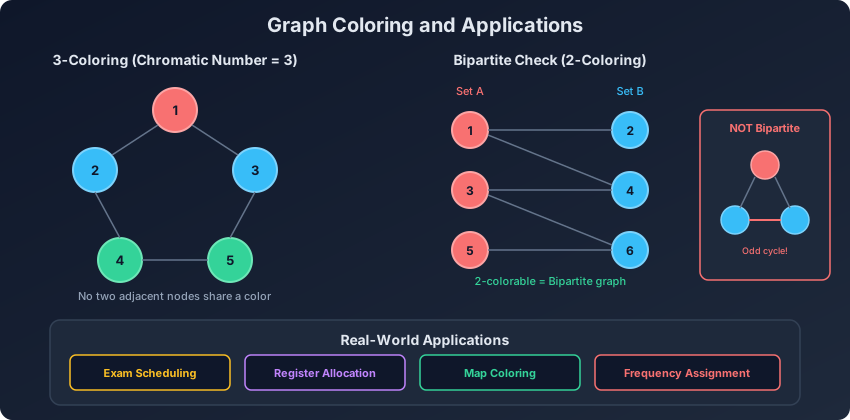
Graph coloring assigns labels (called “colors”) to graph vertices such that no two adjacent vertices share the same color. The minimum number of colors needed is called the chromatic number. While finding the exact chromatic number is NP-hard, practical algorithms and special cases (like bipartite graphs) make graph coloring one of the most useful graph concepts.

The Chromatic Number

The chromatic number of a graph G, written as the Greek letter chi(G), is the smallest number of colors needed to properly color G. Some facts:

• A graph with no edges has chromatic number 1
• A graph with at least one edge has chromatic number at least 2
• A complete graph K_n has chromatic number n
• A bipartite graph has chromatic number at most 2
• A tree has chromatic number 2 (except single node: 1)
• A cycle of even length has chromatic number 2
• A cycle of odd length has chromatic number 3

Finding the exact chromatic number is NP-hard in general, but we have efficient algorithms for specific cases and good heuristics for the general case.

Greedy Coloring

The greedy coloring algorithm processes vertices one at a time and assigns each vertex the smallest color not used by its already-colored neighbors. It is simple, fast, and always uses at most d+1 colors, where d is the maximum degree of the graph.

def greedy_coloring(graph, num_nodes):
    """
    Greedy graph coloring.
    graph: adjacency list
    Returns: dict mapping node -> color (0-indexed)
    """
    color = [-1] * num_nodes

    for node in range(num_nodes):
        # Find colors used by neighbors
        neighbor_colors = set()
        for neighbor in graph[node]:
            if color[neighbor] != -1:
                neighbor_colors.add(color[neighbor])

        # Assign smallest available color
        c = 0
        while c in neighbor_colors:
            c += 1
        color[node] = c

    num_colors = max(color) + 1 if color else 0
    return color, num_colors

Example

# Petersen-like graph
graph = [
    [1, 4],     # 0
    [0, 2],     # 1
    [1, 3],     # 2
    [2, 4],     # 3
    [3, 0]      # 4
]

colors, num_colors = greedy_coloring(graph, 5)
print(f"Colors used: {num_colors}")  # 3 (for odd cycle)
print(f"Coloring: {colors}")         # [0, 1, 0, 1, 2]

Vertex Ordering Matters

The number of colors greedy uses depends on the vertex ordering. The optimal ordering (that minimizes colors) is hard to find, but some heuristics help:

def greedy_coloring_ordered(graph, num_nodes, order):
    """
    Greedy coloring with a specified vertex ordering.
    Different orderings can produce different numbers of colors.
    """
    color = [-1] * num_nodes

    for node in order:
        neighbor_colors = set()
        for neighbor in graph[node]:
            if color[neighbor] != -1:
                neighbor_colors.add(color[neighbor])

        c = 0
        while c in neighbor_colors:
            c += 1
        color[node] = c

    return color, max(color) + 1


def largest_first_ordering(graph, num_nodes):
    """
    Order vertices by decreasing degree.
    Often produces better colorings.
    """
    degrees = [(len(graph[i]), i) for i in range(num_nodes)]
    degrees.sort(reverse=True)
    return [node for _, node in degrees]


def smallest_last_ordering(graph, num_nodes):
    """
    Smallest-last ordering (Welsh-Powell variant).
    Repeatedly remove the vertex with smallest degree.
    """
    degree = [len(graph[i]) for i in range(num_nodes)]
    remaining = set(range(num_nodes))
    order = []

    while remaining:
        # Find vertex with minimum degree among remaining
        min_node = min(remaining, key=lambda x: degree[x])
        order.append(min_node)
        remaining.remove(min_node)

        # Update degrees
        for neighbor in graph[min_node]:
            if neighbor in remaining:
                degree[neighbor] -= 1

    order.reverse()  # Process in reverse removal order
    return order

Greedy Coloring Guarantees

• Upper bound: At most max_degree + 1 colors (Brooks’ theorem says max_degree colors suffice unless the graph is a complete graph or odd cycle)
• Time: O(V + E)
• Space: O(V)
• Optimality: NOT guaranteed to find the minimum number of colors

Bipartite Check as 2-Coloring

A graph is bipartite if and only if it is 2-colorable. This means we can check bipartiteness by trying to 2-color the graph using BFS.

from collections import deque

def is_bipartite(graph, num_nodes):
    """
    Check if a graph is bipartite using BFS 2-coloring.
    Returns: (is_bipartite, coloring_dict)
    """
    color = [-1] * num_nodes

    for start in range(num_nodes):
        if color[start] != -1:
            continue

        # BFS from this node
        queue = deque([start])
        color[start] = 0

        while queue:
            node = queue.popleft()
            for neighbor in graph[node]:
                if color[neighbor] == -1:
                    color[neighbor] = 1 - color[node]
                    queue.append(neighbor)
                elif color[neighbor] == color[node]:
                    return False, {}

    return True, {i: color[i] for i in range(num_nodes)}

Example

# Bipartite graph (even cycle)
bipartite_graph = [
    [1, 3],  # 0
    [0, 2],  # 1
    [1, 3],  # 2
    [2, 0]   # 3
]

is_bip, coloring = is_bipartite(bipartite_graph, 4)
print(f"Bipartite: {is_bip}")    # True
print(f"Coloring: {coloring}")   # {0: 0, 1: 1, 2: 0, 3: 1}

# Non-bipartite graph (odd cycle: triangle)
non_bipartite = [
    [1, 2],  # 0
    [0, 2],  # 1
    [1, 0]   # 2
]

is_bip, _ = is_bipartite(non_bipartite, 3)
print(f"Bipartite: {is_bip}")  # False (odd cycle)

Why Odd Cycles Break Bipartiteness

A graph is bipartite if and only if it contains no odd-length cycle. Here is the intuition: in a 2-coloring, each edge alternates colors. In a cycle, you alternate colors around the cycle. After an even number of edges, you return to the original color. After an odd number, you need a different color but you are back at the start. Contradiction.

def find_odd_cycle(graph, num_nodes):
    """
    If the graph is not bipartite, find an odd cycle.
    Returns: list of nodes forming the odd cycle, or empty list.
    """
    color = [-1] * num_nodes
    parent = [-1] * num_nodes

    for start in range(num_nodes):
        if color[start] != -1:
            continue

        queue = deque([start])
        color[start] = 0

        while queue:
            node = queue.popleft()
            for neighbor in graph[node]:
                if color[neighbor] == -1:
                    color[neighbor] = 1 - color[node]
                    parent[neighbor] = node
                    queue.append(neighbor)
                elif color[neighbor] == color[node]:
                    # Found odd cycle, reconstruct it
                    cycle = []
                    a, b = node, neighbor

                    path_a = []
                    while a != -1:
                        path_a.append(a)
                        a = parent[a]

                    path_b = []
                    while b != -1:
                        path_b.append(b)
                        b = parent[b]

                    # Find common ancestor
                    set_a = set(path_a)
                    lca = -1
                    for x in path_b:
                        if x in set_a:
                            lca = x
                            break

                    # Build cycle
                    for x in path_a:
                        cycle.append(x)
                        if x == lca:
                            break
                    partial = []
                    for x in path_b:
                        if x == lca:
                            break
                        partial.append(x)
                    partial.reverse()
                    cycle.extend(partial)

                    return cycle

    return []

M-Coloring with Backtracking

When you need exactly the minimum number of colors, or need to check if m colors suffice, use backtracking.

def m_coloring(graph, num_nodes, m):
    """
    Check if the graph can be colored with m colors.
    Uses backtracking.
    Returns: True and the coloring, or False and empty.
    """
    color = [0] * num_nodes

    def is_safe(node, c):
        """Check if color c is safe for node."""
        for neighbor in graph[node]:
            if color[neighbor] == c:
                return False
        return True

    def solve(node):
        if node == num_nodes:
            return True

        for c in range(1, m + 1):
            if is_safe(node, c):
                color[node] = c
                if solve(node + 1):
                    return True
                color[node] = 0

        return False

    if solve(0):
        return True, color[:]
    return False, []

Example

# Can we color this graph with 3 colors?
graph = [
    [1, 2, 3],  # 0
    [0, 2],     # 1
    [0, 1, 3],  # 2
    [0, 2]      # 3
]

possible, coloring = m_coloring(graph, 4, 3)
print(f"3-colorable: {possible}")   # True
print(f"Coloring: {coloring}")      # [1, 2, 3, 2] (one possible solution)

# Find chromatic number
for m in range(1, 5):
    possible, _ = m_coloring(graph, 4, m)
    if possible:
        print(f"Chromatic number: {m}")
        break
# Chromatic number: 3

Optimized Backtracking with Pruning

def m_coloring_optimized(graph, num_nodes, m):
    """
    M-coloring with forward checking and MRV heuristic.
    """
    color = [0] * num_nodes
    available = [set(range(1, m + 1)) for _ in range(num_nodes)]

    def select_next():
        """MRV: select uncolored node with fewest available colors."""
        best_node = -1
        min_colors = m + 1

        for i in range(num_nodes):
            if color[i] == 0 and len(available[i]) < min_colors:
                min_colors = len(available[i])
                best_node = i

        return best_node

    colored_count = 0

    def solve():
        nonlocal colored_count

        if colored_count == num_nodes:
            return True

        node = select_next()
        if node == -1 or not available[node]:
            return False

        for c in list(available[node]):
            color[node] = c
            colored_count += 1

            # Forward check: remove c from neighbors' available
            removed = []
            valid = True
            for neighbor in graph[node]:
                if color[neighbor] == 0 and c in available[neighbor]:
                    available[neighbor].remove(c)
                    removed.append(neighbor)
                    if not available[neighbor]:
                        valid = False
                        break

            if valid and solve():
                return True

            # Undo
            color[node] = 0
            colored_count -= 1
            for neighbor in removed:
                available[neighbor].add(c)

        return False

    if solve():
        return True, color[:]
    return False, []

Complexity

• Time: O(m^V) worst case (trying all color assignments)
• Space: O(V) for the recursion stack
• With pruning, much faster in practice but still exponential worst case

Application: Exam Scheduling

Schedule exams so that no student has two exams at the same time. Students taking common courses create conflicts.

def schedule_exams(courses, conflicts):
    """
    Schedule exams with minimum time slots.
    courses: list of course names
    conflicts: list of (course_i, course_j) pairs
    Returns: dict mapping course -> time slot
    """
    n = len(courses)
    graph = [[] for _ in range(n)]

    for i, j in conflicts:
        graph[i].append(j)
        graph[j].append(i)

    # Use greedy coloring with largest-first ordering
    order = largest_first_ordering(graph, n)
    colors, num_slots = greedy_coloring_ordered(graph, n, order)

    schedule = {}
    for i, course in enumerate(courses):
        schedule[course] = f"Slot {colors[i] + 1}"

    print(f"Minimum time slots needed: {num_slots}")
    return schedule


# Example
courses = ["Math", "Physics", "CS", "English", "Chemistry"]
conflicts = [(0, 1), (0, 2), (1, 3), (2, 3), (2, 4)]

schedule = schedule_exams(courses, conflicts)
for course, slot in schedule.items():
    print(f"  {course}: {slot}")

Application: Register Allocation

Compilers use graph coloring to assign variables to CPU registers. Build an interference graph where variables that are live at the same time are connected. Color the graph with k colors (k = number of registers). If k colors are not enough, some variables must be “spilled” to memory.

def allocate_registers(variables, interferences, num_registers):
    """
    Assign variables to registers using graph coloring.
    variables: list of variable names
    interferences: list of (var_i, var_j) pairs that cannot share a register
    num_registers: number of available registers
    Returns: dict mapping variable -> register, list of spilled variables
    """
    n = len(variables)
    graph = [[] for _ in range(n)]

    for i, j in interferences:
        graph[i].append(j)
        graph[j].append(i)

    possible, coloring = m_coloring(graph, n, num_registers)

    if possible:
        allocation = {}
        for i, var in enumerate(variables):
            allocation[var] = f"R{coloring[i]}"
        return allocation, []
    else:
        # Greedy color, spill variables needing extra colors
        colors, num_colors = greedy_coloring(graph, n)
        allocation = {}
        spilled = []

        for i, var in enumerate(variables):
            if colors[i] < num_registers:
                allocation[var] = f"R{colors[i] + 1}"
            else:
                spilled.append(var)
                allocation[var] = "MEMORY"

        return allocation, spilled

Application: Map Coloring

The famous Four Color Theorem guarantees any planar graph (like a map) can be colored with at most 4 colors.

def color_map(regions, borders):
    """
    Color a map with minimum colors (at most 4 for planar graphs).
    regions: list of region names
    borders: list of (region_i, region_j) pairs sharing a border
    """
    n = len(regions)
    graph = [[] for _ in range(n)]

    for i, j in borders:
        graph[i].append(j)
        graph[j].append(i)

    # Try 4-coloring (guaranteed to work for planar graphs)
    possible, coloring = m_coloring(graph, n, 4)

    color_names = ['Red', 'Blue', 'Green', 'Yellow']
    result = {}
    for i, region in enumerate(regions):
        result[region] = color_names[coloring[i] - 1]

    return result


# Example: Map of some states
regions = ["CA", "OR", "WA", "NV", "AZ"]
borders = [(0, 1), (0, 3), (0, 4), (1, 2), (1, 3), (3, 4)]

colored_map = color_map(regions, borders)
for region, color in colored_map.items():
    print(f"  {region}: {color}")

Application: Frequency Assignment

In wireless networks, adjacent towers cannot use the same frequency. This is graph coloring where colors represent frequencies.

def assign_frequencies(towers, interferences, available_frequencies):
    """
    Assign frequencies to cell towers avoiding interference.
    """
    n = len(towers)
    graph = [[] for _ in range(n)]

    for i, j in interferences:
        graph[i].append(j)
        graph[j].append(i)

    colors, num_freq = greedy_coloring(graph, n)

    if num_freq > available_frequencies:
        print(f"WARNING: Need {num_freq} frequencies but only "
              f"{available_frequencies} available")

    assignment = {}
    for i, tower in enumerate(towers):
        freq = (colors[i] % available_frequencies) + 1
        assignment[tower] = f"Freq-{freq}"

    return assignment

Edge Coloring

Edge coloring assigns colors to edges so no two edges sharing a vertex have the same color. Vizing’s theorem says every graph can be edge-colored with at most max_degree + 1 colors.

def edge_coloring_greedy(num_nodes, edges):
    """
    Greedy edge coloring.
    Returns: dict mapping edge -> color
    """
    edge_colors = {}
    node_edge_colors = [set() for _ in range(num_nodes)]

    for u, v in edges:
        # Find smallest color not used by either endpoint
        used = node_edge_colors[u] | node_edge_colors[v]
        c = 0
        while c in used:
            c += 1

        edge_colors[(u, v)] = c
        node_edge_colors[u].add(c)
        node_edge_colors[v].add(c)

    return edge_colors

Complexity Summary

Algorithm	Time	Colors Used	Optimal?
Greedy	O(V + E)	At most d+1	No
2-coloring (bipartite check)	O(V + E)	2	Yes (for bipartite)
M-coloring (backtracking)	O(m^V)	Exactly m	Yes
Welsh-Powell (largest first)	O(V + E)	Often near optimal	No

Practice Problems

1. Is Graph Bipartite? (LeetCode 785) - 2-coloring with BFS
2. Possible Bipartition (LeetCode 886) - 2-coloring with constraints
3. Flower Planting With No Adjacent (LeetCode 1042) - 4-coloring (guaranteed)
4. Graph Coloring (backtracking judges) - M-coloring
5. Exam Scheduling - Graph coloring application
6. Course Schedule with Conflicts - Chromatic number variant

Key Takeaways

Graph coloring assigns labels to vertices so no two adjacent vertices share a label. The chromatic number (minimum colors needed) is NP-hard to compute in general, but greedy coloring gives a fast O(V + E) heuristic using at most max_degree + 1 colors. Bipartite checking is 2-coloring and runs in O(V + E) with BFS. For exact solutions, backtracking with pruning works for small graphs. Real-world applications include scheduling (courses/exams to time slots), register allocation (variables to CPU registers), map coloring, and frequency assignment in wireless networks.