ETL vs ELT Pipelines Explained With Examples

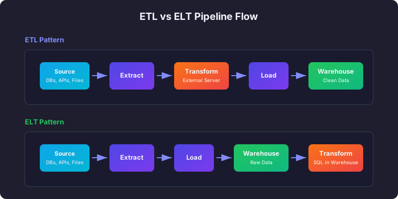
Every data pipeline does three things: extract data from a source, transform it into something useful, and load it into a destination. The question is the order. ETL transforms before loading. ELT loads first and transforms inside the destination. This seemingly small difference changes your architecture, your tooling, and your team’s workflow.

ETL — Extract, Transform, Load

In ETL, data is pulled from source systems, transformed on a separate compute layer, and then loaded into the destination.

Source → [Extract] → Staging Server → [Transform] → [Load] → Warehouse

How it works

1. Extract — connect to source systems (databases, APIs, files) and pull raw data.
2. Transform — on a dedicated processing server, clean the data, apply business rules, join datasets, aggregate values, and reshape into the target schema.
3. Load — write the final, transformed data into the destination warehouse or database.

Example: ETL with Python and Pandas

import pandas as pd
from sqlalchemy import create_engine

# 1. Extract — read from source database
source_engine = create_engine("postgresql://source_db:5432/app")
orders = pd.read_sql("SELECT * FROM orders WHERE date > '2026-01-01'", source_engine)
customers = pd.read_sql("SELECT * FROM customers", source_engine)

# 2. Transform — clean and enrich
orders["total_usd"] = orders["total"] * orders["exchange_rate"]
orders = orders.dropna(subset=["customer_id"])
enriched = orders.merge(customers[["id", "segment", "country"]], 
                         left_on="customer_id", right_on="id")
daily_revenue = enriched.groupby(["date", "segment", "country"])["total_usd"].sum().reset_index()

# 3. Load — write to warehouse
warehouse_engine = create_engine("postgresql://warehouse:5432/analytics")
daily_revenue.to_sql("daily_revenue", warehouse_engine, if_exists="replace", index=False)

The transformation happens outside the warehouse, on whatever machine runs this script.

When ETL makes sense

• Sensitive data — you need to mask, hash, or filter PII before it reaches the warehouse.
• Legacy systems — the destination database has limited compute power (on-premise, old RDBMS).
• Complex transformations — heavy ML feature engineering or image/text processing that SQL cannot express.
• Cost control — warehouse compute is expensive and you want to minimize what runs there.

ELT — Extract, Load, Transform

In ELT, raw data is loaded into the warehouse first, and transformations happen inside it using SQL.

Source → [Extract] → [Load] → Warehouse → [Transform in SQL] → Clean Tables

How it works

1. Extract — same as ETL, pull data from sources.
2. Load — dump raw data directly into the warehouse in staging tables, preserving the original structure.
3. Transform — write SQL inside the warehouse to clean, join, and reshape data into analytics-ready tables.

Example: ELT with dbt

After raw data is loaded into the warehouse by an ingestion tool like Fivetran or Airbyte, dbt handles the transformation step:

-- models/staging/stg_orders.sql
WITH source AS (
    SELECT * FROM {{ source('raw', 'orders') }}
),

cleaned AS (
    SELECT
        id AS order_id,
        customer_id,
        total * exchange_rate AS total_usd,
        created_at::date AS order_date
    FROM source
    WHERE customer_id IS NOT NULL
)

SELECT * FROM cleaned

-- models/marts/daily_revenue.sql
WITH orders AS (
    SELECT * FROM {{ ref('stg_orders') }}
),

customers AS (
    SELECT * FROM {{ ref('stg_customers') }}
)

SELECT
    o.order_date,
    c.segment,
    c.country,
    SUM(o.total_usd) AS revenue
FROM orders o
JOIN customers c ON o.customer_id = c.customer_id
GROUP BY 1, 2, 3

The warehouse does the heavy lifting. No separate compute needed.

When ELT makes sense

• Cloud warehouses — Snowflake, BigQuery, and Redshift can scale compute elastically. Let them do the work.
• Iterative analysis — raw data in the warehouse means analysts can explore and transform without waiting for engineers.
• Version-controlled transformations — dbt models are SQL files in Git, testable and reviewable.
• Schema flexibility — you can reload and retransform without re-extracting from the source.

Side-by-side comparison

Dimension	ETL	ELT
Transform location	External server / processing layer	Inside the warehouse
Raw data in warehouse	No — only cleaned data arrives	Yes — raw data lands first
Warehouse compute cost	Lower — transforms happen elsewhere	Higher — warehouse does the work
Flexibility	Lower — must re-extract to re-transform	Higher — raw data allows re-transformation
Latency	Higher — extra hop through transform layer	Lower — fewer steps
Tooling	Python, Spark, custom scripts	dbt, SQL, warehouse features
Data privacy	Easier — filter PII before loading	Harder — raw PII lands in warehouse
Best for	Legacy systems, complex transforms, PII	Cloud warehouses, SQL-heavy teams

The industry shift toward ELT

Before 2015, most pipelines were ETL. Warehouses were expensive, disk-based, on-premise systems. You minimized what you loaded because storage and compute cost real money.

Cloud warehouses changed the economics. BigQuery charges per query scan. Snowflake separates storage from compute and lets you scale each independently. Storage became cheap. Compute became elastic. Suddenly it was cheaper to load everything raw and transform inside the warehouse than to maintain a separate Spark cluster for transformations.

This shift gave rise to tools like:

• Fivetran / Airbyte — handle the EL (extract and load) step with pre-built connectors.
• dbt — handles the T (transform) step with SQL models, tests, and documentation.
• Snowflake / BigQuery / Redshift — provide the compute for transformations.

The “modern data stack” is essentially an ELT stack: Fivetran → Snowflake → dbt → Looker.

Hybrid approaches

In practice, most teams use a mix:

• ELT for structured data — database tables, API responses, CSV files. Load raw, transform in SQL.
• ETL for unstructured data — images, logs, PDFs. Transform externally with Python or Spark, then load the results.
• Streaming + batch — real-time events flow through Kafka for immediate use, then land in the warehouse for batch transformation.

The choice is not religious. Use whichever pattern fits the data source, the sensitivity requirements, and the team’s skills.

Next steps

• Data Warehouse Concepts — understand star schemas and dimensional modeling.
• What Is Apache Airflow? — orchestrate your ETL/ELT pipelines.
• Batch vs Stream Processing — when nightly runs are not fast enough.