Multi-Source BFS: Simultaneous Search from Multiple Starting Points

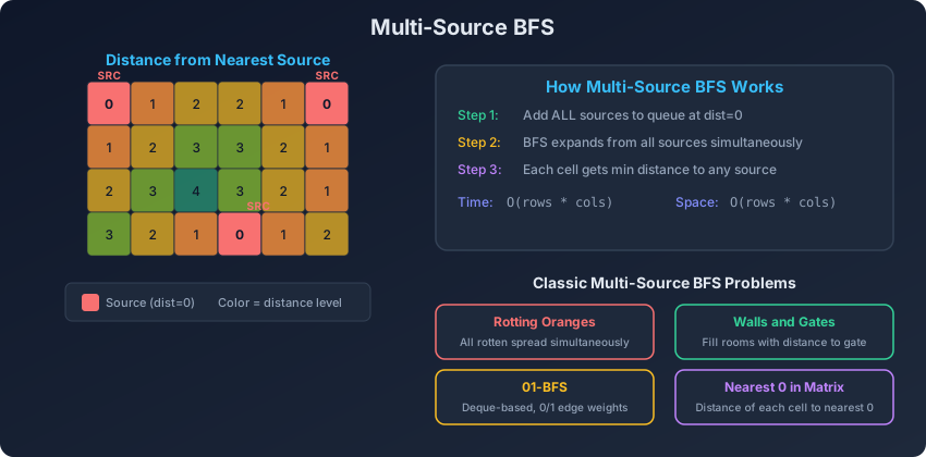
Standard BFS starts from a single source and finds the shortest distance to all reachable nodes. Multi-source BFS starts from multiple sources simultaneously, finding the shortest distance from each cell to its nearest source. The trick is simple but powerful: add all source nodes to the queue at the beginning with distance 0, then run regular BFS.

This is equivalent to adding a virtual super-source node connected to all actual sources with zero-weight edges, then running single-source BFS from that super-source. But we do not need to actually create the super-source; we just initialize the queue with all sources.

The Core Pattern

from collections import deque

def multi_source_bfs(grid, sources):
    """
    Multi-source BFS on a grid.
    sources: list of (row, col) starting positions
    Returns: 2D distance grid where each cell has the
             distance to its nearest source
    """
    rows, cols = len(grid), len(grid[0])
    dist = [[-1] * cols for _ in range(rows)]
    queue = deque()

    # Initialize: all sources at distance 0
    for r, c in sources:
        dist[r][c] = 0
        queue.append((r, c))

    # Standard BFS from here
    while queue:
        r, c = queue.popleft()
        for dr, dc in [(0, 1), (0, -1), (1, 0), (-1, 0)]:
            nr, nc = r + dr, c + dc
            if (0 <= nr < rows and 0 <= nc < cols
                    and dist[nr][nc] == -1):
                dist[nr][nc] = dist[r][c] + 1
                queue.append((nr, nc))

    return dist

Why This Works

When BFS processes nodes level by level, each level corresponds to a distance. In multi-source BFS, level 0 contains all sources. Level 1 contains all cells that are exactly 1 step from their nearest source. Level 2 contains cells exactly 2 steps from their nearest source, and so on. Each cell is visited exactly once, and the first time it is visited gives the correct minimum distance to any source.

Why Not Run Single-Source BFS Multiple Times?

Running single-source BFS from each source separately gives O(S * V) time where S is the number of sources and V is the number of cells. Multi-source BFS does it in O(V) total, because each cell is processed exactly once regardless of the number of sources.

Problem 1: Rotting Oranges (LeetCode 994)

Every minute, fresh oranges adjacent to rotten ones become rotten. Return the minimum minutes until no fresh orange remains, or -1 if impossible.

def oranges_rotting(grid):
    """
    LeetCode 994: Rotting Oranges.
    0 = empty, 1 = fresh orange, 2 = rotten orange
    Returns minimum minutes, or -1 if impossible.
    """
    rows, cols = len(grid), len(grid[0])
    queue = deque()
    fresh_count = 0

    # Find all rotten oranges (sources) and count fresh
    for r in range(rows):
        for c in range(cols):
            if grid[r][c] == 2:
                queue.append((r, c, 0))  # (row, col, time)
            elif grid[r][c] == 1:
                fresh_count += 1

    if fresh_count == 0:
        return 0

    max_time = 0

    while queue:
        r, c, time = queue.popleft()

        for dr, dc in [(0, 1), (0, -1), (1, 0), (-1, 0)]:
            nr, nc = r + dr, c + dc
            if (0 <= nr < rows and 0 <= nc < cols
                    and grid[nr][nc] == 1):
                grid[nr][nc] = 2  # Mark as rotten
                fresh_count -= 1
                max_time = time + 1
                queue.append((nr, nc, time + 1))

    return max_time if fresh_count == 0 else -1

Example

grid = [
    [2, 1, 1],
    [1, 1, 0],
    [0, 1, 1]
]
print(oranges_rotting(grid))  # 4

# Minute 0: rotten at (0,0)
# Minute 1: (0,1) and (1,0) rot
# Minute 2: (0,2) and (1,1) rot
# Minute 3: (2,1) rots
# Minute 4: (2,2) rots

Problem 2: Walls and Gates (LeetCode 286)

Fill each empty room with the distance to its nearest gate. Walls are -1 and gates are 0.

def walls_and_gates(rooms):
    """
    LeetCode 286: Walls and Gates.
    -1 = wall, 0 = gate, INF = empty room (2147483647)
    Modifies rooms in-place.
    """
    if not rooms:
        return

    INF = 2147483647
    rows, cols = len(rooms), len(rooms[0])
    queue = deque()

    # Find all gates (sources)
    for r in range(rows):
        for c in range(cols):
            if rooms[r][c] == 0:
                queue.append((r, c))

    # Multi-source BFS from all gates
    while queue:
        r, c = queue.popleft()
        for dr, dc in [(0, 1), (0, -1), (1, 0), (-1, 0)]:
            nr, nc = r + dr, c + dc
            if (0 <= nr < rows and 0 <= nc < cols
                    and rooms[nr][nc] == INF):
                rooms[nr][nc] = rooms[r][c] + 1
                queue.append((nr, nc))

Example

INF = 2147483647
rooms = [
    [INF, -1,  0, INF],
    [INF, INF, INF, -1],
    [INF, -1, INF, -1],
    [0,   -1, INF, INF]
]

walls_and_gates(rooms)
for row in rooms:
    print([x if x != INF else 'INF' for x in row])
# [3, -1, 0, 1]
# [2, 2, 1, -1]
# [1, -1, 2, -1]
# [0, -1, 3, 4]

Problem 3: 01 Matrix (LeetCode 542)

Find the distance of each cell to the nearest 0.

def update_matrix(mat):
    """
    LeetCode 542: 01 Matrix.
    Find distance of each cell to nearest 0.
    """
    rows, cols = len(mat), len(mat[0])
    dist = [[float('inf')] * cols for _ in range(rows)]
    queue = deque()

    # All 0 cells are sources
    for r in range(rows):
        for c in range(cols):
            if mat[r][c] == 0:
                dist[r][c] = 0
                queue.append((r, c))

    while queue:
        r, c = queue.popleft()
        for dr, dc in [(0, 1), (0, -1), (1, 0), (-1, 0)]:
            nr, nc = r + dr, c + dc
            if (0 <= nr < rows and 0 <= nc < cols
                    and dist[nr][nc] > dist[r][c] + 1):
                dist[nr][nc] = dist[r][c] + 1
                queue.append((nr, nc))

    return dist

Problem 4: Shortest Bridge (LeetCode 934)

Find the shortest bridge between two islands.

def shortest_bridge(grid):
    """
    LeetCode 934: Shortest Bridge.
    Find minimum flips to connect two islands.
    """
    rows, cols = len(grid), len(grid[0])
    visited = [[False] * cols for _ in range(rows)]
    queue = deque()

    # Step 1: Find first island using DFS, add its border to queue
    def dfs(r, c):
        if (r < 0 or r >= rows or c < 0 or c >= cols
                or visited[r][c] or grid[r][c] == 0):
            return
        visited[r][c] = True
        queue.append((r, c, 0))  # All cells of first island
        dfs(r + 1, c)
        dfs(r - 1, c)
        dfs(r, c + 1)
        dfs(r, c - 1)

    # Find any cell of the first island
    found = False
    for r in range(rows):
        if found:
            break
        for c in range(cols):
            if grid[r][c] == 1:
                dfs(r, c)
                found = True
                break

    # Step 2: Multi-source BFS from first island to reach second
    while queue:
        r, c, dist = queue.popleft()
        for dr, dc in [(0, 1), (0, -1), (1, 0), (-1, 0)]:
            nr, nc = r + dr, c + dc
            if (0 <= nr < rows and 0 <= nc < cols
                    and not visited[nr][nc]):
                if grid[nr][nc] == 1:
                    return dist  # Reached second island
                visited[nr][nc] = True
                queue.append((nr, nc, dist + 1))

    return -1

01-BFS: The Deque Technique

When edge weights are only 0 or 1, you can use a deque instead of a priority queue. Push 0-weight edges to the front and 1-weight edges to the back. This gives O(V + E) time instead of O((V + E) log V) for Dijkstra.

from collections import deque

def bfs_01(graph, source, num_nodes):
    """
    0-1 BFS using a deque.
    graph: dict mapping node -> list of (neighbor, weight)
    where weight is 0 or 1
    Returns: distance array
    """
    dist = [float('inf')] * num_nodes
    dist[source] = 0
    dq = deque([source])

    while dq:
        node = dq.popleft()

        for neighbor, weight in graph[node]:
            new_dist = dist[node] + weight
            if new_dist < dist[neighbor]:
                dist[neighbor] = new_dist
                if weight == 0:
                    dq.appendleft(neighbor)  # Front for 0-cost
                else:
                    dq.append(neighbor)      # Back for 1-cost

    return dist

Example: Minimum Cost to Make Valid Path (LeetCode 1368)

Grid cells have arrows. Moving along the arrow costs 0, changing direction costs 1.

def min_cost(grid):
    """
    LeetCode 1368: Minimum Cost to Make at Least One Valid Path.
    1=right, 2=left, 3=down, 4=up
    """
    rows, cols = len(grid), len(grid[0])
    # Direction mappings: right, left, down, up
    dir_map = {1: (0, 1), 2: (0, -1), 3: (1, 0), 4: (-1, 0)}
    all_dirs = [(0, 1), (0, -1), (1, 0), (-1, 0)]

    dist = [[float('inf')] * cols for _ in range(rows)]
    dist[0][0] = 0
    dq = deque([(0, 0)])

    while dq:
        r, c = dq.popleft()

        for dr, dc in all_dirs:
            nr, nc = r + dr, c + dc
            if 0 <= nr < rows and 0 <= nc < cols:
                # Cost 0 if this direction matches the arrow
                arrow_dr, arrow_dc = dir_map[grid[r][c]]
                cost = 0 if (dr == arrow_dr and dc == arrow_dc) else 1
                new_dist = dist[r][c] + cost

                if new_dist < dist[nr][nc]:
                    dist[nr][nc] = new_dist
                    if cost == 0:
                        dq.appendleft((nr, nc))
                    else:
                        dq.append((nr, nc))

    return dist[rows - 1][cols - 1]

Multi-Source BFS with State

Sometimes the BFS state is more than just position. You might track position plus some additional state like keys collected.

def shortest_path_with_keys(grid):
    """
    Shortest path to collect all keys in a grid.
    State: (row, col, keys_bitmask)
    """
    rows, cols = len(grid), len(grid[0])
    queue = deque()
    total_keys = 0

    # Find start and count keys
    for r in range(rows):
        for c in range(cols):
            if grid[r][c] == '@':
                queue.append((r, c, 0, 0))  # row, col, keys, dist
            elif grid[r][c].islower():
                total_keys += 1

    all_keys = (1 << total_keys) - 1
    visited = set()

    while queue:
        r, c, keys, dist = queue.popleft()

        if keys == all_keys:
            return dist

        state = (r, c, keys)
        if state in visited:
            continue
        visited.add(state)

        for dr, dc in [(0, 1), (0, -1), (1, 0), (-1, 0)]:
            nr, nc = r + dr, c + dc
            if 0 <= nr < rows and 0 <= nc < cols:
                cell = grid[nr][nc]
                if cell == '#':
                    continue
                new_keys = keys
                if cell.islower():
                    new_keys |= (1 << (ord(cell) - ord('a')))
                if cell.isupper() and not (keys & (1 << (ord(cell.lower()) - ord('a')))):
                    continue  # Locked door, no key

                new_state = (nr, nc, new_keys)
                if new_state not in visited:
                    queue.append((nr, nc, new_keys, dist + 1))

    return -1

Complexity Analysis

All multi-source BFS problems on grids have the same complexity:

Aspect	Complexity
Time	O(rows * cols)
Space	O(rows * cols)

The number of sources does not affect the time complexity because each cell is still visited at most once. This is the key advantage over running single-source BFS from each source.

Common Patterns and Tips

1. Identify the sources: The first step is always identifying what the sources are. In rotting oranges, sources are rotten oranges. In walls and gates, sources are gates. In 01 matrix, sources are 0 cells.

2. Initialize all sources at distance 0: Add all sources to the queue before starting the BFS loop.

3. Check if multi-source helps: If you need “distance to nearest X” for every cell, multi-source BFS from all X cells is the right approach.

4. 01-BFS for 0/1 weights: When edge costs are 0 or 1, use a deque. Appendleft for 0-cost, append for 1-cost. This avoids the log factor of a priority queue.

Practice Problems

1. Rotting Oranges (LeetCode 994) - Multi-source BFS with time tracking
2. Walls and Gates (LeetCode 286) - Distance to nearest gate
3. 01 Matrix (LeetCode 542) - Distance to nearest zero
4. Shortest Bridge (LeetCode 934) - DFS + multi-source BFS
5. As Far from Land as Possible (LeetCode 1162) - Distance from water to nearest land
6. Map of Highest Peak (LeetCode 1765) - Multi-source distance assignment
7. Minimum Cost to Make Valid Path (LeetCode 1368) - 01-BFS

Key Takeaways

Multi-source BFS is a simple but powerful technique: initialize the queue with all sources at distance 0, then run standard BFS. It computes the minimum distance from every cell to its nearest source in O(V) time. The 01-BFS variant handles 0/1 edge weights using a deque, giving Dijkstra-level results at BFS speed. Whenever a problem asks for “nearest” or “minimum distance to closest X,” think multi-source BFS.