Pandas Window Functions: Rolling, Expanding, and EWM

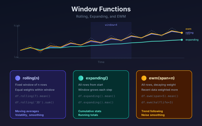
Window functions compute statistics over a sliding, expanding, or weighted subset of your data. They are essential for time-series analysis, finance, sensor data, and any scenario where you need smoothed or cumulative metrics without collapsing your rows.

Rolling Windows

rolling(window) creates a fixed-size sliding window. At each row, it looks back window rows and applies an aggregation.

import pandas as pd
import numpy as np

# simulated daily stock prices
dates = pd.date_range('2026-01-01', periods=10, freq='D')
prices = pd.Series(
    [100, 102, 101, 105, 107, 103, 108, 110, 109, 112],
    index=dates
)

# 3-day moving average
prices.rolling(window=3).mean()

2026-01-01       NaN
2026-01-02       NaN
2026-01-03    101.00
2026-01-04    102.67
2026-01-05    104.33
2026-01-06    105.00
2026-01-07    106.00
2026-01-08    107.00
2026-01-09    109.00
2026-01-10    110.33

The first two rows are NaN because the window needs 3 values. Use min_periods to allow partial windows:

prices.rolling(window=3, min_periods=1).mean()
# now row 1 uses just [100], row 2 uses [100, 102], etc.

Common Rolling Aggregations

df = pd.DataFrame({'price': prices})

df['ma_7']    = df['price'].rolling(7).mean()      # moving average
df['std_7']   = df['price'].rolling(7).std()        # rolling volatility
df['max_5']   = df['price'].rolling(5).max()        # rolling high
df['min_5']   = df['price'].rolling(5).min()        # rolling low
df['sum_3']   = df['price'].rolling(3).sum()        # rolling sum

Time-Based Windows

When your index is a DatetimeIndex, you can specify the window as a time offset instead of a fixed number of rows. This handles missing dates correctly.

# window of 3 calendar days (not 3 rows)
prices.rolling('3D').mean()

Expanding Windows

expanding() uses every row from the start up to the current row. The window grows with each step, giving you cumulative statistics.

prices.expanding().mean()   # cumulative mean
prices.expanding().max()    # running maximum
prices.expanding().std()    # cumulative std deviation

2026-01-01    100.00    # mean of [100]
2026-01-02    101.00    # mean of [100, 102]
2026-01-03    101.00    # mean of [100, 102, 101]
2026-01-04    102.00    # mean of first 4 values
...

Practical Use: Cumulative Return

daily_returns = prices.pct_change()
cumulative_return = (1 + daily_returns).expanding().apply(np.prod) - 1

print(cumulative_return.iloc[-1])  # total return over the period

Exponentially Weighted Moving (EWM)

ewm() assigns exponentially decreasing weights to older observations. Recent data points matter more. This is widely used in finance for smoothing noisy signals.

# span=5 means the "center of mass" is roughly 5 periods
prices.ewm(span=5).mean()

The three ways to control decay:

# these are equivalent ways to set the same decay rate
prices.ewm(span=9).mean()       # span: decay = 2/(span+1)
prices.ewm(com=4).mean()        # center of mass
prices.ewm(halflife=3).mean()   # half-life in periods

Comparing All Three Windows

df = pd.DataFrame({'price': prices})
df['rolling_5']   = df['price'].rolling(5).mean()
df['expanding']   = df['price'].expanding().mean()
df['ewm_5']       = df['price'].ewm(span=5).mean()

print(df.round(2))

• Rolling: reacts to recent changes, flat weight within window.
• Expanding: smoothest, dominated by historical data.
• EWM: reacts quickly to recent shifts, weights decay smoothly.

GroupBy + Rolling

A common real-world need: compute a rolling average per category. Chain groupby() before rolling().

sales = pd.DataFrame({
    'date': pd.date_range('2026-01-01', periods=12, freq='D').tolist() * 2,
    'store': ['A'] * 12 + ['B'] * 12,
    'revenue': np.random.randint(100, 500, 24)
})

sales['rolling_avg_3'] = (
    sales
    .groupby('store')['revenue']
    .transform(lambda x: x.rolling(3, min_periods=1).mean())
)

The transform call ensures the result has the same index as the original DataFrame. Each store gets its own independent rolling window.

GroupBy + Expanding for Running Totals

sales['cumulative_rev'] = (
    sales
    .groupby('store')['revenue']
    .transform(lambda x: x.expanding().sum())
)

Custom Window Functions

Use .apply() on a rolling object to run any function over each window.

# rolling coefficient of variation (std / mean)
def coeff_variation(window):
    return window.std() / window.mean() if window.mean() != 0 else 0

prices.rolling(5).apply(coeff_variation, raw=False)

Setting raw=True passes a NumPy array instead of a Series, which is faster when you do not need the index:

# rolling geometric mean (faster with raw=True)
from scipy.stats import gmean

prices.rolling(5).apply(gmean, raw=True)

Using rolling with Multiple Columns

df = pd.DataFrame({
    'high': [105, 108, 107, 112, 110],
    'low':  [98,  100, 99,  103, 102],
})

# rolling average true range
df['range'] = df['high'] - df['low']
df['avg_range_3'] = df['range'].rolling(3).mean()

Performance Tips

1. Prefer built-in aggregations (mean, sum, std) over .apply(). Built-ins run in C and are 10-100x faster.
2. Use raw=True in .apply() when you do not need the Series index.
3. Use engine='numba' for custom functions on large datasets:

from numba import njit

@njit
def custom_mean(values):
    return values.sum() / len(values)

prices.rolling(5).apply(custom_mean, raw=True, engine='numba')

4. Set min_periods explicitly to control NaN behavior at the edges of your data.

Quick Reference

Method	Window Size	Weight Distribution	Best For
rolling(n)	Fixed n rows	Equal	Moving averages, volatility
expanding()	All rows so far	Equal	Cumulative stats, running totals
ewm(span=n)	All rows (decaying)	Exponential decay	Trend following, smoothing noise

Window functions let you analyze trends, smooth noise, and compute running statistics without losing row-level granularity. Start with rolling() for fixed-window analysis, use expanding() for cumulative metrics, and reach for ewm() when recent observations should dominate.