Binary Tree Views: Left, Right, Top & Bottom

Tree “view” problems ask: what do you see when you look at a tree from a particular direction? They are a staple of coding interviews and all follow a similar pattern — BFS with some form of level or column tracking. Once you understand the framework, all four views become straightforward.

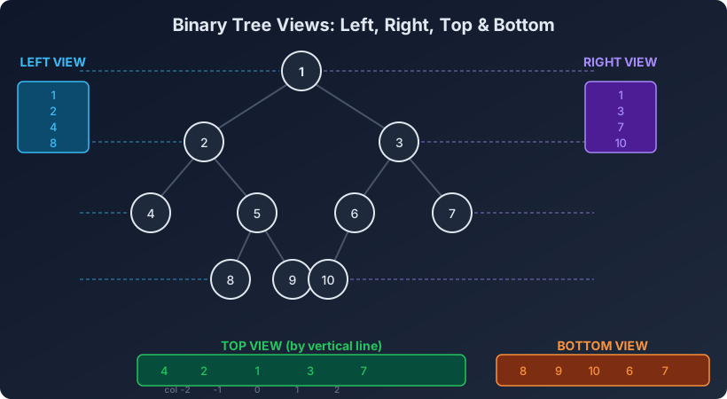
The common tree for all examples

We will use this tree throughout:

         1
        / \
       2   3
      / \   / \
     4   5 6   7
        / \   /
       8   9 10

Left view

The left view shows the first node visible at each level when looking from the left side.

Level 0: [1]       → see 1
Level 1: [2, 3]    → see 2
Level 2: [4, 5, 6, 7] → see 4
Level 3: [8, 9, 10]   → see 8

Left view: [1, 2, 4, 8]

BFS approach

from collections import deque

def left_view(root):
    """Return the left view of a binary tree."""
    if not root:
        return []

    result = []
    queue = deque([root])

    while queue:
        level_size = len(queue)
        for i in range(level_size):
            node = queue.popleft()

            # First node at this level
            if i == 0:
                result.append(node.val)

            if node.left:
                queue.append(node.left)
            if node.right:
                queue.append(node.right)

    return result

DFS approach (recursive)

def left_view_dfs(root):
    """Left view using DFS — first node at each depth."""
    result = []

    def dfs(node, depth):
        if node is None:
            return

        # If this is the first node at this depth
        if depth == len(result):
            result.append(node.val)

        # Visit left first (so left nodes are seen first)
        dfs(node.left, depth + 1)
        dfs(node.right, depth + 1)

    dfs(root, 0)
    return result

The trick: depth == len(result) means no node has been added for this level yet. Since we visit left before right, the leftmost node wins.

Right view

The right view shows the last node at each level — what you see looking from the right.

Level 0: [1]       → see 1
Level 1: [2, 3]    → see 3
Level 2: [4, 5, 6, 7] → see 7
Level 3: [8, 9, 10]   → see 10

Right view: [1, 3, 7, 10]

BFS approach

def right_view(root):
    """Return the right view of a binary tree."""
    if not root:
        return []

    result = []
    queue = deque([root])

    while queue:
        level_size = len(queue)
        for i in range(level_size):
            node = queue.popleft()

            # Last node at this level
            if i == level_size - 1:
                result.append(node.val)

            if node.left:
                queue.append(node.left)
            if node.right:
                queue.append(node.right)

    return result

DFS approach

def right_view_dfs(root):
    """Right view using DFS — visit right first."""
    result = []

    def dfs(node, depth):
        if node is None:
            return

        if depth == len(result):
            result.append(node.val)

        # Visit right first (so rightmost nodes are seen first)
        dfs(node.right, depth + 1)
        dfs(node.left, depth + 1)

    dfs(root, 0)
    return result

The only difference from left view DFS: we visit right before left.

Vertical order traversal (foundation for top/bottom views)

Before tackling top and bottom views, we need to understand vertical columns.

Assign each node a column number:

• Root is at column 0
• Left child is at column - 1
• Right child is at column + 1

         1 (col 0)
        / \
   (col-1) 2   3 (col 1)
      / \   / \
(col-2) 4  5 6  7 (col 2)
       (col 0)(col 0)(col 1)
       / \   /
      8   9 10
   (col-1)(col 1)(col 0... wait)

Let me be precise:

Node 1:  col=0,  level=0
Node 2:  col=-1, level=1
Node 3:  col=1,  level=1
Node 4:  col=-2, level=2
Node 5:  col=0,  level=2
Node 6:  col=0,  level=2
Node 7:  col=2,  level=2
Node 8:  col=-1, level=3
Node 9:  col=1,  level=3
Node 10: col=-1, level=3  (wait, 6's left child? col=0-1=-1? No.)

Let me correct — node 10 is the left child of node 7 (col=2), so node 10 is at col=1, level=3.

Vertical order traversal implementation

from collections import defaultdict, deque

def vertical_order_traversal(root):
    """Return vertical order traversal of binary tree."""
    if not root:
        return []

    # Map: column → list of (row, value)
    columns = defaultdict(list)
    min_col = max_col = 0

    queue = deque([(root, 0, 0)])  # (node, col, row)

    while queue:
        node, col, row = queue.popleft()
        columns[col].append((row, node.val))
        min_col = min(min_col, col)
        max_col = max(max_col, col)

        if node.left:
            queue.append((node.left, col - 1, row + 1))
        if node.right:
            queue.append((node.right, col + 1, row + 1))

    result = []
    for col in range(min_col, max_col + 1):
        # Sort by row, then by value for same position
        col_vals = sorted(columns[col])
        result.append([val for _, val in col_vals])

    return result

Top view

The top view shows the first node seen at each vertical column when looking from above. For each column, it is the node with the smallest row (highest in the tree).

Column -2: [4]           → see 4
Column -1: [2, 8]        → see 2 (row 1 < row 3)
Column  0: [1, 5, 6]     → see 1 (row 0)
Column  1: [3, 9]        → see 3 (row 1 < row 3)
Column  2: [7]           → see 7

Top view: [4, 2, 1, 3, 7]

def top_view(root):
    """Return the top view of a binary tree."""
    if not root:
        return []

    # For each column, store the first node seen (BFS guarantees top-first)
    column_map = {}
    min_col = max_col = 0

    queue = deque([(root, 0)])  # (node, column)

    while queue:
        node, col = queue.popleft()

        # Only record the first node at each column
        if col not in column_map:
            column_map[col] = node.val

        min_col = min(min_col, col)
        max_col = max(max_col, col)

        if node.left:
            queue.append((node.left, col - 1))
        if node.right:
            queue.append((node.right, col + 1))

    return [column_map[col] for col in range(min_col, max_col + 1)]

BFS naturally processes nodes top-to-bottom, so the first node we encounter at each column is the topmost one.

Bottom view

The bottom view shows the last node at each vertical column when looking from below.

Column -2: [4]           → see 4
Column -1: [2, 8]        → see 8 (row 3 > row 1)
Column  0: [1, 5, 6]     → see 5 or 6 (both row 2, leftmost in BFS: 5)
Column  1: [3, 9]        → see 9 (row 3 > row 1)
Column  2: [7]           → see 7

Bottom view: [4, 8, 5, 9, 7]  (or 6 instead of 5 depending on convention)

def bottom_view(root):
    """Return the bottom view of a binary tree."""
    if not root:
        return []

    # For each column, keep overwriting (last one wins)
    column_map = {}
    min_col = max_col = 0

    queue = deque([(root, 0)])

    while queue:
        node, col = queue.popleft()

        # Always overwrite — last (deepest) node wins
        column_map[col] = node.val

        min_col = min(min_col, col)
        max_col = max(max_col, col)

        if node.left:
            queue.append((node.left, col - 1))
        if node.right:
            queue.append((node.right, col + 1))

    return [column_map[col] for col in range(min_col, max_col + 1)]

The difference from top view: instead of checking if col not in column_map, we always overwrite. The last node at each column (deepest, or rightmost at same depth due to BFS order) is the bottom view node.

Boundary view (bonus)

The boundary of a binary tree is: left boundary + leaves + right boundary (in reverse). This combines left view, leaf detection, and right view.

def boundary_of_binary_tree(root):
    """Return the boundary values of a binary tree."""
    if not root:
        return []

    result = [root.val]

    # Left boundary (excluding root and leaves)
    def left_boundary(node):
        if node is None or (node.left is None and node.right is None):
            return
        result.append(node.val)
        if node.left:
            left_boundary(node.left)
        else:
            left_boundary(node.right)

    # All leaves (left to right)
    def leaves(node):
        if node is None:
            return
        if node.left is None and node.right is None:
            result.append(node.val)
            return
        leaves(node.left)
        leaves(node.right)

    # Right boundary (excluding root and leaves, in reverse)
    def right_boundary(node):
        if node is None or (node.left is None and node.right is None):
            return
        if node.right:
            right_boundary(node.right)
        else:
            right_boundary(node.left)
        result.append(node.val)  # append after recursion = reverse

    left_boundary(root.left)
    leaves(root.left)
    leaves(root.right)
    right_boundary(root.right)

    return result

Diagonal view

Another variation: group nodes by their diagonal. A node at diagonal d has its right child at diagonal d and left child at diagonal d + 1.

def diagonal_traversal(root):
    """Return diagonal traversal of binary tree."""
    if not root:
        return []

    diagonals = defaultdict(list)
    queue = deque([(root, 0)])

    while queue:
        node, d = queue.popleft()
        diagonals[d].append(node.val)

        if node.left:
            queue.append((node.left, d + 1))
        if node.right:
            queue.append((node.right, d))  # same diagonal

    return [diagonals[d] for d in sorted(diagonals)]

Performance comparison

All view problems share the same complexity:

Operation	Time	Space
Left view (BFS)	O(n)	O(w) where w = max width
Right view (BFS)	O(n)	O(w)
Top view	O(n)	O(n)
Bottom view	O(n)	O(n)
Vertical order	O(n log n)	O(n)
Left view (DFS)	O(n)	O(h)

The BFS approaches use O(w) space for the queue (w = maximum width of the tree). The column-based approaches use O(n) for the hash map.

Common patterns and tips

1. Left/Right view: Track the first/last node at each level (row)
2. Top/Bottom view: Track the first/last node at each column
3. BFS gives level order for free — use level_size = len(queue) to process level by level
4. Column assignment: left child = col - 1, right child = col + 1
5. For top view, BFS order guarantees correctness — first encounter at a column is the topmost
6. For bottom view, keep overwriting — last encounter at a column is the bottommost

Practice problems

1. Binary Tree Right Side View (LeetCode 199) — Right view
2. Vertical Order Traversal (LeetCode 987) — Columns + sorting
3. Binary Tree Level Order Traversal (LeetCode 102) — Foundation for views
4. Top View of Binary Tree (GeeksforGeeks) — First at each column
5. Bottom View of Binary Tree (GeeksforGeeks) — Last at each column
6. Left View of Binary Tree (GeeksforGeeks) — First at each level
7. Boundary of Binary Tree (LeetCode 545) — Combines multiple views
8. Find Largest Value in Each Tree Row (LeetCode 515)

Key takeaways

• All view problems are variations of BFS with tracking by level or column
• Left/Right views track by level (row number)
• Top/Bottom views track by column (vertical line number)
• BFS naturally processes top-to-bottom, so first-at-column = top view
• DFS can also solve left/right views by visiting the correct child first
• Vertical order traversal is the most general — top and bottom views are specializations