Data Structures Comparison Guide: When to Use What
A comprehensive comparison of data structures — arrays vs linked lists, hash maps vs trees vs tries, heaps vs BSTs, stacks vs queues, sets vs Bloom filters, with decision flowcharts and complexity tables.
What you'll learn
- ✓When to choose Array vs LinkedList vs Deque
- ✓When to choose HashMap vs TreeMap vs Trie
- ✓When to choose Heap vs Sorted Array vs BST
- ✓When to choose Stack vs Queue vs Priority Queue
- ✓When to choose Set vs BitSet vs Bloom Filter
- ✓When to use adjacency list vs adjacency matrix for graphs
- ✓A decision flowchart for choosing the right data structure
Prerequisites
- •Familiar with basic data structures and Big-O notation
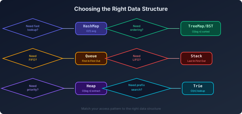
Knowing how a data structure works is step one. The real skill is knowing when to use it. In interviews and system design, the first question is always the same: “Which data structure fits this problem?”
This guide gives you head-to-head comparisons, complexity tables, and a decision flowchart. Bookmark it. Come back to it before interviews. Use it as your mental index into the world of data structures.
1. Array vs LinkedList vs Deque
These are the three fundamental sequential containers. Each makes a different trade-off.
When to use each
| Operation | Array | LinkedList | Deque (double-ended queue) |
|---|---|---|---|
| Access by index | O(1) | O(n) | O(1) (array-based) |
| Insert/delete at end | O(1) amortised | O(1) if tail pointer | O(1) |
| Insert/delete at front | O(n) | O(1) | O(1) |
| Insert/delete in middle | O(n) | O(1) if you have the node | O(n) |
| Memory overhead | Low (contiguous) | High (pointers per node) | Medium |
| Cache performance | Excellent | Poor (scattered memory) | Good |
Array (contiguous in memory):
┌───┬───┬───┬───┬───┐
│ 3 │ 1 │ 4 │ 1 │ 5 │ → CPU cache loves this
└───┴───┴───┴───┴───┘
LinkedList (scattered in memory):
[3|→] … [1|→] … [4|→] … [1|→] [5|∅]
↑ cache miss ↑ cache miss ↑ cache miss
Decision guide
- Default choice: Array. It is the fastest, simplest, and most cache-friendly.
- Need O(1) front insertion/deletion: Deque.
- Need O(1) middle insertion with a pointer to the node: LinkedList.
- Building a queue: Deque.
- Implementing LRU cache: LinkedList (for O(1) move-to-front) + HashMap.
Real-world: arrays back 90% of all data structures. Even “linked” structures like trees are often stored in arrays for cache performance (binary heap = array).
2. HashMap vs TreeMap vs Trie
All three map keys to values, but with very different performance profiles.
Comparison table
| Operation | HashMap | TreeMap (Balanced BST) | Trie |
|---|---|---|---|
| Insert | O(1) avg | O(log n) | O(L) where L = key length |
| Lookup | O(1) avg | O(log n) | O(L) |
| Delete | O(1) avg | O(log n) | O(L) |
| Find min/max | O(n) | O(log n) | Depends |
| Range query (keys in [a,b]) | O(n) | O(log n + k) | Depends |
| Prefix search | O(n) | O(n) | O(L) |
| Ordered iteration | O(n log n) to sort | O(n) in-order | O(total chars) |
| Space | O(n) | O(n) | O(alphabet * total nodes) |
Decision guide
- Need fast lookup by exact key: HashMap. It is the default.
- Need keys in sorted order or range queries: TreeMap.
- Need prefix search (“find all words starting with ‘pre’”): Trie.
- Keys are integers in a small range: plain array (index = key).
# HashMap: O(1) lookup
from collections import defaultdict
word_count = defaultdict(int)
for word in words:
    word_count[word] += 1

# TreeMap equivalent in Python: SortedDict from sortedcontainers
from sortedcontainers import SortedDict
sd = SortedDict()
sd["apple"] = 1
sd["banana"] = 2
# sd.irange("a", "b") → keys in range ["a", "b"]

# Trie: O(L) prefix search
class TrieNode:
    def __init__(self):
        self.children = {}
        self.is_end = False
Interview tip: when someone says “design autocomplete,” the answer is Trie (or a similar prefix structure). When they say “design a cache,” the answer starts with HashMap.
3. Heap vs Sorted Array vs BST
All three maintain some notion of order, but each is optimised for different access patterns.
Comparison table
| Operation | Min-Heap | Sorted Array | Balanced BST |
|---|---|---|---|
| Find min/max | O(1) | O(1) | O(log n) |
| Insert | O(log n) | O(n) | O(log n) |
| Delete min/max | O(log n) | O(1) or O(n) | O(log n) |
| Delete arbitrary | O(n) | O(n) | O(log n) |
| Search | O(n) | O(log n) | O(log n) |
| Find k-th element | O(n) | O(1) | O(log n) with augmentation |
| Space | O(n) | O(n) | O(n) |
Decision guide
- Need the min or max repeatedly: Heap. It is purpose-built for this.
- Need both min and max: two heaps (min-heap + max-heap), or a balanced BST.
- Data is static, need k-th element: Sorted array.
- Need fast insert + delete + search: Balanced BST.
- Building a priority queue: Heap.
import heapq

# Heap: perfect for "give me the smallest element"
pq = []
heapq.heappush(pq, 5)
heapq.heappush(pq, 2)
heapq.heappush(pq, 8)
print(heapq.heappop(pq))  # 2

# Sorted array: perfect for binary search
arr = [1, 3, 5, 7, 9]
import bisect
idx = bisect.bisect_left(arr, 5)  # O(log n) search
Classic interview problem: “Find the median of a stream” → use two heaps (max-heap for lower half, min-heap for upper half).
4. Stack vs Queue vs Priority Queue
Three containers with different access policies.
| Property | Stack | Queue | Priority Queue |
|---|---|---|---|
| Order | LIFO | FIFO | By priority |
| Push | O(1) | O(1) | O(log n) |
| Pop | O(1) | O(1) | O(log n) |
| Peek | O(1) | O(1) | O(1) |
| Use case | Undo, parsing, DFS | BFS, scheduling | Dijkstra, task scheduling |
When to use each
- Stack: problems involving nesting (parentheses, HTML tags), most recent element (undo/redo), DFS (explicit stack), monotonic stack (next greater element).
- Queue: BFS (level-by-level traversal), task scheduling (FIFO fairness), rate limiting (sliding window of requests).
- Priority Queue: always need the best/worst element (Dijkstra’s algorithm, merge k sorted lists, event simulation), scheduling by priority (OS task scheduler).
Stack:          Queue:          Priority Queue:
┌───┐          ┌───────────┐    ┌───┐
│ 3 │ ← top    │ 1 2 3 4 5 │    │ 1 │ ← min (always the best)
│ 2 │          └───────────┘    │ 3 │
│ 1 │          front → out      │ 5 │
└───┘                           │ 7 │
top → out                       └───┘
5. Set vs BitSet vs Bloom Filter
All three answer the question “is this element in the collection?”
| Property | HashSet | BitSet | Bloom Filter |
|---|---|---|---|
| Insert | O(1) | O(1) | O(k) (k hash functions) |
| Lookup | O(1) | O(1) | O(k) |
| Delete | O(1) | O(1) | Not supported |
| False positives | No | No | Yes (tunable) |
| False negatives | No | No | No |
| Space for n elements | O(n) | O(max_value) bits | O(n) bits (much less than HashSet) |
| Works with | Any hashable type | Integers in a known range | Any hashable type |
Decision guide
- Default membership test: HashSet.
- Elements are integers in [0, N] and N is manageable: BitSet (extremely space-efficient).
- Space is critical and false positives are acceptable: Bloom Filter.
# HashSet: general purpose
seen = set()
seen.add("apple")
print("apple" in seen)  # True

# BitSet: for integer elements in a known range
class BitSet:
    def __init__(self, size):
        self.bits = [0] * ((size >> 5) + 1)

    def add(self, x):
        self.bits[x >> 5] |= (1 << (x & 31))

    def contains(self, x):
        return bool(self.bits[x >> 5] & (1 << (x & 31)))

bs = BitSet(1000)
bs.add(42)
print(bs.contains(42))  # True
print(bs.contains(43))  # False
Interview example: “Check if a character has been seen” with only lowercase letters → use a 26-bit integer as a BitSet.
6. Graph Representations: Adjacency List vs Matrix
| Property | Adjacency List | Adjacency Matrix |
|---|---|---|
| Space | O(V + E) | O(V^2) |
| Check if edge exists | O(degree) | O(1) |
| Iterate neighbours | O(degree) | O(V) |
| Add edge | O(1) | O(1) |
| Remove edge | O(degree) | O(1) |
| Best for | Sparse graphs (E << V^2) | Dense graphs (E close to V^2) |
Decision guide
- Most real-world graphs (social networks, road maps): Adjacency list. They are sparse.
- Dense graphs or need O(1) edge lookup: Adjacency matrix.
- Weighted edges: Adjacency list with (neighbour, weight) tuples, or matrix with weights as values.
# Adjacency list (most common)
from collections import defaultdict
graph = defaultdict(list)
graph[0].append(1)
graph[0].append(2)
graph[1].append(2)

# Adjacency matrix
n = 5
matrix = [[0] * n for _ in range(n)]
matrix[0][1] = 1  # edge from 0 to 1
matrix[0][2] = 1  # edge from 0 to 2
Comprehensive Comparison Table
Here is every major data structure at a glance:
| Data Structure | Insert | Delete | Search | Min/Max | Ordered | Space |
|---|---|---|---|---|---|---|
| Array | O(n)* | O(n) | O(n) | O(n) | No | O(n) |
| Sorted Array | O(n) | O(n) | O(log n) | O(1) | Yes | O(n) |
| LinkedList | O(1)** | O(1)** | O(n) | O(n) | No | O(n) |
| Stack | O(1) | O(1) | O(n) | O(n) | LIFO | O(n) |
| Queue | O(1) | O(1) | O(n) | O(n) | FIFO | O(n) |
| HashMap | O(1) | O(1) | O(1) | O(n) | No | O(n) |
| TreeMap/BST | O(log n) | O(log n) | O(log n) | O(log n) | Yes | O(n) |
| Heap | O(log n) | O(log n) | O(n) | O(1) | Partial | O(n) |
| Trie | O(L) | O(L) | O(L) | - | Lexicographic | O(AL*n) |
| Segment Tree | O(log n) | - | O(log n) | O(log n) | - | O(n) |
| Fenwick Tree | O(log n) | - | O(log n) | - | - | O(n) |
*Array append is O(1) amortised. **LinkedList O(1) with pointer to node.
The “Which Data Structure?” Decision Flowchart
When you face a new problem, ask these questions in order:
-
Do I need key-value mapping?
├─ Yes → Need ordering? → Yes → TreeMap
│ → No → HashMap
└─ No → Continue
-
Do I need to maintain order of insertion?
├─ LIFO → Stack
├─ FIFO → Queue
├─ By priority → Heap / Priority Queue
└─ No specific order → Continue
-
Do I need fast membership testing?
├─ Elements are small integers → BitSet
├─ Approximate OK → Bloom Filter
└─ Exact → HashSet
-
Do I need sorted data?
├─ Static (no inserts) → Sorted Array
├─ Dynamic → Balanced BST / TreeSet
└─ No → Array or LinkedList
-
Is it a graph problem?
├─ Sparse → Adjacency List
└─ Dense → Adjacency Matrix
-
Need range queries?
├─ Static → Sparse Table (min/max) or Prefix Sum (sum)
└─ Dynamic → Segment Tree or Fenwick Tree
Real-World Mapping
| Real-world system | Primary data structure | Why |
|---|---|---|
| Database index | B+ Tree | O(log n) on disk with high branching factor |
| In-memory cache (Redis) | Hash table + skip list | O(1) lookup + O(log n) sorted ops |
| Search engine index | Inverted index (hash map) | O(1) term lookup |
| DNS resolver cache | Hash table | O(1) domain lookup |
| Undo/redo system | Stack | LIFO matches undo order |
| Print queue | Queue | FIFO fairness |
| Autocomplete | Trie | O(L) prefix matching |
| Event scheduler | Priority queue (heap) | Always process earliest event |
| Social network | Adjacency list graph | Sparse connections |
| Route planner | Weighted graph + Dijkstra | Shortest path |
Interview Tips
When the interviewer says… you should think…
- “Find the k most frequent…” → HashMap (count) + Heap (top k)
- “Find if a path exists…” → Graph + BFS/DFS
- “Design an LRU cache…” → HashMap + Doubly LinkedList
- “Find the median in a stream…” → Two Heaps
- “Implement autocomplete…” → Trie
- “Check for balanced parentheses…” → Stack
- “Find shortest path…” → Graph + BFS (unweighted) or Dijkstra (weighted)
- “Range sum queries with updates…” → Segment Tree or Fenwick Tree
The meta-strategy
- Start with the simplest structure (array, hash map). Most problems can be solved with these.
- Upgrade only when needed. Need ordering? Switch from HashMap to TreeMap. Need fast min? Add a Heap.
- Combine structures for complex requirements. LRU cache = HashMap + LinkedList. Median of stream = two Heaps.
Recap
Choosing the right data structure is the most impactful decision in any coding problem:
- Arrays are the default — fast, simple, cache-friendly
- HashMaps provide O(1) lookup for unordered data
- TreeMaps/BSTs maintain sorted order with O(log n) operations
- Heaps give you the min/max in O(1) with O(log n) updates
- Tries excel at prefix-based operations on strings
- Stacks, queues, and priority queues enforce specific access orders
- Graph representations depend on density
The right data structure makes the right algorithm obvious. The wrong data structure makes every algorithm painful.
Next steps
See these data structures in action in real systems: DSA in Real Systems. For interview preparation strategy, see Problem Solving Framework.
Questions or feedback? Email codeloomdevv@gmail.com.
Related articles
- DSA DSA Interview Checklist: 75 Must-Know Problems
The complete DSA interview checklist — 75 essential problems organized by pattern, study schedules for 4, 8, and 12 weeks, a pattern recognition framework, and what interviewers actually look for.
- DSA Graph Interview Patterns: Complete Guide
Master the top 20 graph interview patterns with a BFS vs DFS decision flowchart, Union-Find strategies, grid vs adjacency list trade-offs, and template code.
- DSA Linked List Interview Patterns: Complete Guide
Master the top 15 linked list interview patterns — dummy node, fast-slow pointers, reversal, merge, partition, and more. Includes common mistakes, a time complexity cheatsheet, and a decision flowchart.
- DSA String Interview Patterns: Complete Guide
A complete guide to string interview patterns — top 20 patterns, two-pointer on strings, frequency map technique, sliding window template, when to use Trie vs HashMap, common mistakes, and a complexity cheatsheet.